Introduction to Statistical Modeling with SAS/STAT Software: Test of Hypotheses

Test of Hypotheses

Consider a general linear hypothesis of the form $\text{[math]}$ , where $\text{[math]}$ is a $\text{[math]}$ matrix. It is assumed that $\text{[math]}$ is such that this hypothesis is linearly consistent—that is, that there exists some $\text{[math]}$ for which $\text{[math]}$ . This is always the case if $\text{[math]}$ is in the column space of $\text{[math]}$ , if $\text{[math]}$ has full row rank, or if $\text{[math]}$ ; the latter is the most common case. Since many linear models have a rank-deficient $\text{[math]}$ matrix, the question arises whether the hypothesis is testable. The idea of testability of a hypothesis is—not surprisingly—connected to the concept of estimability as introduced previously. The hypothesis $\text{[math]}$ is testable if it consists of estimable functions.

There are two important approaches to testing hypotheses in statistical applications—the reduction principle and the linear inference approach. The reduction principle states that the validity of the hypothesis can be inferred by comparing a suitably chosen summary statistic between the model at hand and a reduced model in which the constraint $\text{[math]}$ is imposed. The linear inference approach relies on the fact that $\text{[math]}$ is an estimator of $\text{[math]}$ and its stochastic properties are known, at least approximately. A test statistic can then be formed using $\text{[math]}$ , and its behavior under the restriction $\text{[math]}$ can be ascertained.

The two principles lead to identical results in certain—for example, least squares estimation in the classical linear model. In more complex situations the two approaches lead to similar but not identical results. This is the case, for example, when weights or unequal variances are involved, or when $\text{[math]}$ is a nonlinear estimator.

Reduction Tests

The two main reduction principles are the sum of squares reduction test and the likelihood ratio test. The test statistic in the former is proportional to the difference of the residual sum of squares between the reduced model and the full model. The test statistic in the likelihood ratio test is proportional to the difference of the log likelihoods between the full and reduced models. To fix these ideas, suppose that you are fitting the model $\text{[math]}$ , where $\text{[math]}$ . Suppose that $\text{[math]}$ denotes the residual sum of squares in this model and that $\text{[math]}$ is the residual sum of squares in the model for which $\text{[math]}$ holds. Then under the hypothesis the ratio

$\text{[math]}$

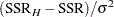follows a chi-square distribution with degrees of freedom equal to the rank of $\text{[math]}$ . Maybe surprisingly, the residual sum of squares in the full model is distributed independently of this quantity, so that under the hypothesis,

$\text{[math]}$

follows an $\text{[math]}$ distribution with $\text{[math]}$ numerator and $\text{[math]}$ denominator degrees of freedom. Note that the quantity in the denominator of the $\text{[math]}$ statistic is a particular estimator of $\text{[math]}$ —namely, the unbiased moment-based estimator that is customarily associated with least squares estimation. It is also the restricted maximum likelihood estimator of $\text{[math]}$ if $\text{[math]}$ is normally distributed.

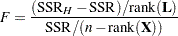
In the case of the likelihood ratio test, suppose that $\text{[math]}$ denotes the log likelihood evaluated at the ML estimators. Also suppose that $\text{[math]}$ denotes the log likelihood in the model for which $\text{[math]}$ holds. Then under the hypothesis the statistic

$\text{[math]}$

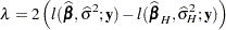follows approximately a chi-square distribution with degrees of freedom equal to the rank of $\text{[math]}$ . In the case of a normally distributed response, the log-likelihood function can be profiled with respect to $\text{[math]}$ . The resulting profile log likelihood is

$\text{[math]}$

and the likelihood ratio test statistic becomes

$\text{[math]}$

The preceding expressions show that, in the case of normally distributed data, both reduction principles lead to simple functions of the residual sums of squares in two models. As Pawitan (2001, p. 151) puts it, there is, however, an important difference not in the computations but in the statistical content. The least squares principle, where sum of squares reduction tests are widely used, does not require a distributional specification. Assumptions about the distribution of the data are added to provide a framework for confirmatory inferences, such as the testing of hypotheses. This framework stems directly from the assumption about the data’s distribution, or from the sampling distribution of the least squares estimators. The likelihood principle, on the other hand, requires a distributional specification at the outset. Inference about the parameters is implicit in the model; it is the result of further computations following the estimation of the parameters. In the least squares framework, inference about the parameters is the result of further assumptions.

Linear Inference

The principle of linear inference is to formulate a test statistic for $\text{[math]}$ that builds on the linearity of the hypothesis about $\text{[math]}$ . For many models that have linear components, the estimator $\text{[math]}$ is also linear in $\text{[math]}$ . It is then simple to establish the distributional properties of $\text{[math]}$ based on the distributional assumptions about $\text{[math]}$ or based on large-sample arguments. For example, $\text{[math]}$ might be a nonlinear estimator, but it is known to asymptotically follow a normal distribution; this is the case in many nonlinear and generalized linear models.

If the sampling distribution or the asymptotic distribution of $\text{[math]}$ is normal, then one can easily derive quadratic forms with known distributional properties. For example, if the random vector $\text{[math]}$ is distributed as $\text{[math]}$ , then $\text{[math]}$ follows a chi-square distribution with $\text{[math]}$ degrees of freedom and noncentrality parameter $\text{[math]}$ , provided that $\text{[math]}$ .

In the classical linear model, suppose that $\text{[math]}$ is deficient in rank and that 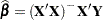$\text{[math]}$ is a solution to the normal equations. Then, if the errors are normally distributed,

$\text{[math]}$

Because $\text{[math]}$ is testable, $\text{[math]}$ is estimable, and thus 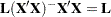$\text{[math]}$ , as established in the previous section. Hence,

$\text{[math]}$

The conditions for a chi-square distribution of the quadratic form

$\text{[math]}$

are thus met, provided that

$\text{[math]}$

This condition is obviously met if $\text{[math]}$ is of full rank. The condition is also met if $\text{[math]}$ is a reflexive inverse (a $\text{[math]}$ -inverse) of $\text{[math]}$ .

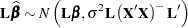
The test statistic to test the linear hypothesis $\text{[math]}$ is thus

$\text{[math]}$

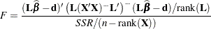and it follows an $\text{[math]}$ distribution with $\text{[math]}$ numerator and $\text{[math]}$ denominator degrees of freedom under the hypothesis.

This test statistic looks very similar to the $\text{[math]}$ statistic for the sum of squares reduction test. This is no accident. If the model is linear and parameters are estimated by ordinary least squares, then you can show that the quadratic form $\text{[math]}$ equals the differences in the residual sum of squares, $\text{[math]}$ , where $\text{[math]}$ is obtained as the residual sum of squares from OLS estimation in a model that satisfies $\text{[math]}$ . However, this correspondence between the two test formulations does not apply when a different estimation principle is used. For example, assume that $\text{[math]}$ and that $\text{[math]}$ is estimated by generalized least squares:

$\text{[math]}$

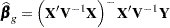The construction of $\text{[math]}$ matrices associated with hypotheses in SAS/STAT software is frequently based on the properties of the $\text{[math]}$ matrix, not of $\text{[math]}$ . In other words, the construction of the $\text{[math]}$ matrix is governed only by the design. A sum of squares reduction test for $\text{[math]}$ that uses the generalized residual sum of squares 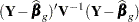$\text{[math]}$ is not identical to a linear hypothesis test with the statistic

$\text{[math]}$

Furthermore, $\text{[math]}$ is usually unknown and must be estimated as well. The estimate for $\text{[math]}$ depends on the model, and imposing a constraint on the model would change the estimate. The asymptotic distribution of the statistic $\text{[math]}$ is a chi-square distribution. However, in practical applications the $\text{[math]}$ distribution with $\text{[math]}$ numerator and $\text{[math]}$ denominator degrees of freedom is often used because it provides a better approximation to the sampling distribution of $\text{[math]}$ in finite samples. The computation of the denominator degrees of freedom $\text{[math]}$ , however, is a matter of considerable discussion. A number of methods have been proposed and are implemented in various forms in SAS/STAT (see, for example, the degrees-of-freedom methods in the MIXED and GLIMMIX procedures).