| The LIFEREG Procedure |
| Probability Plotting |
Probability plots are useful tools for the display and analysis of lifetime data. Probability plots use an inverse distribution scale so that a cumulative distribution function (CDF) plots as a straight line. A nonparametric estimate of the CDF of the lifetime data will plot approximately as a straight line, thus providing a visual assessment of goodness of fit.
You can use the PROBPLOT statement in PROC LIFEREG to create probability plots of data that are complete, right censored, interval censored, or a combination of censoring types (arbitrarily censored). A line representing the maximum likelihood fit from the MODEL statement and pointwise parametric confidence bands for the cumulative probabilities are also included in the plot.
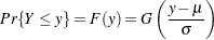
A random variable  belongs to a location-scale family of distributions if its CDF
  is of the form
 |
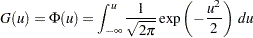
where  is the location parameter and
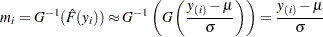
  is the scale parameter. Here,
  is a CDF that cannot depend on any unknown parameters, and is the CDF of if
  and
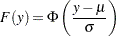
and  . For example, if is a normal random variable with mean and standard deviation ,
 |
and
 |
The normal, extreme-value, and logistic distributions are location-scale models. The three-parameter gamma distribution is a location-scale model if the shape parameter  is fixed. If
  has a lognormal, Weibull, or log-logistic distribution, then
  has a distribution that is a location-scale model. Probability plots are constructed for lognormal, Weibull, and log-logistic distributions by using instead of in the plots.
Let  be ordered observations of a random sample with distribution function
  . A probability plot is a plot of the points
  against
  , where
  is an estimate of the CDF
 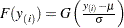 . The nonparametric CDF estimates
  are sometimes called plotting positions. The axis on which the points
  are plotted is usually labeled with a probability scale (the scale of ).
If is one of the location-scale distributions, then  is the lifetime; otherwise, the log of the lifetime is used to transform the distribution to a location-scale model.
If the data actually have the stated distribution, then  ,
,
 |
and points  should fall approximately in a straight line.
There are several ways to compute the nonparametric CDF estimates used in probability plots from lifetime data. These are discussed in the next two sections.
Complete and Right-Censored Data
The censoring times must be taken into account when you compute plotting positions for right-censored data. The modified Kaplan-Meier method described in the following section is the default method for computing nonparametric CDF estimates for display on probability plots. Refer to Abernethy (1996), Meeker and Escobar (1998), and Nelson (1982) for discussions of the methods described in the following sections.
Expected Ranks, Kaplan-Meier, and Modified Kaplan-Meier Methods
Let be ordered observations of a random sample including failure times and censor times. Order the data in increasing order. Label all the data with reverse ranks  , with
  . For the lifetime (not censoring time) corresponding to reverse rank , compute the survival function estimate
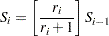 |
with  . The expected rank plotting position is computed as
  . The option PPOS=EXPRANK specifies the expected rank plotting position.
For the Kaplan-Meier method,
 |
The Kaplan-Meier plotting position is then computed as  . The option PPOS=KM specifies the Kaplan-Meier plotting position.
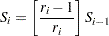
For the modified Kaplan-Meier method, use
 |
where  is computed from the Kaplan-Meier formula with . The plotting position is then computed as
  . The option PPOS=MKM specifies the modified Kaplan-Meier plotting position. If the PPOS option is not specified, the modified Kaplan-Meier plotting position is used as the default method.
For complete samples,  for the expected rank method,
  for the Kaplan-Meier method, and
  for the modified Kaplan-Meier method. If the largest observation is a failure for the Kaplan-Meier estimator, then
  and the point is not plotted.
Median Ranks
Let be ordered observations of a random sample including failure times and censor times. A failure order number  is assigned to the ith failure:
  , where
  . The increment
  is initially 1 and is modified when a censoring time is encountered in the ordered sample. The new increment is computed as
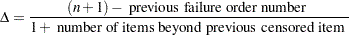 |
The plotting position is computed for the  th failure time as
 |
For complete samples, the failure order number is equal to , the order of the failure in the sample. In this case, the preceding equation for is an approximation of the median plotting position computed as the median of the ith-order statistic from the uniform distribution on (0, 1). In the censored case, is not necessarily an integer, but the preceding equation still provides an approximation to the median plotting position. The PPOS=MEDRANK option specifies the median rank plotting position.
Arbitrarily Censored Data
The LIFEREG procedure can create probability plots for data that consist of combinations of exact, left-censored, right-censored, and interval-censored lifetimes—that is, arbitrarily censored data. The LIFEREG procedure uses an iterative algorithm developed by Turnbull (1976) to compute a nonparametric maximum likelihood estimate of the cumulative distribution function for the data. Since the technique is maximum likelihood, standard errors of the cumulative probability estimates are computed from the inverse of the associated Fisher information matrix. This algorithm is an example of the expectation-maximization (EM) algorithm. The default initial estimate assigns equal probabilities to each interval. You can specify different initial values with the PROBLIST= option. Convergence is determined if the change in the log likelihood between two successive iterations is less than delta, where the default value of delta is  . You can specify a different value for delta with the TOLLIKE= option. Iterations will be terminated if the algorithm does not converge after a fixed number of iterations. The default maximum number of iterations is 1000. Some data might require more iterations for convergence. You can specify the maximum allowed number of iterations with the MAXITEM= option in the PROBPLOT statement. The iteration history of the log likelihood is displayed if you specify the ITPRINTEM option. The iteration history of the estimated interval probabilities are also displayed if you specify both options ITPRINTEM and PRINTPROBS.
If an interval probability is smaller than a tolerance ( by default) after convergence, the probability is set to zero, the interval probabilities are renormalized so that they add to one, and iterations are restarted. Usually the algorithm converges in just a few more iterations. You can change the default value of the tolerance with the TOLPROB= option. You can specify the NOPOLISH option to avoid setting small probabilities to zero and restarting the algorithm.
If you specify the ITPRINTEM option, a table summarizing the Turnbull estimate of the interval probabilities is displayed. The columns labeled "Reduced Gradient" and "Lagrange Multiplier" are used in checking final convergence of the maximum likelihood estimate. The Lagrange multipliers must all be greater than or equal to zero, or the solution is not maximum likelihood. Refer to Gentleman and Geyer (1994) for more details of the convergence checking. Also refer to Meeker and Escobar (1998, Chapter 3) for more information.
See Example 48.6 for an illustration.
Nonparametric Confidence Intervals
You can use the PPOUT option in the PROBPLOT statement to create a table containing the nonparametric CDF estimates computed by the selected method, Kaplan-Meier CDF estimates, standard errors of the Kaplan-Meier estimator, and nonparametric confidence limits for the CDF. The confidence limits are either pointwise or simultaneous, depending on the value of the NPINTERVALS= option in the PROBPLOT statement. The method used in the LIFEREG procedure for computation of approximate pointwise and simultaneous confidence intervals for cumulative failure probabilities relies on the Kaplan-Meier estimator of the cumulative distribution function of failure time and approximate standard deviation of the Kaplan-Meier estimator. For the case of arbitrarily censored data, the Turnbull algorithm, discussed previously, provides an extension of the Kaplan-Meier estimator. Both the Kaplan-Meier and the Turnbull estimators provide an estimate of the standard error of the CDF estimator,  , that is used in computing confidence intervals.
Pointwise Confidence Intervals
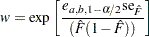
Approximate  pointwise confidence intervals are computed as in Meeker and Escobar (1998, Section 3.6) as
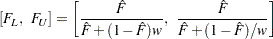 |
where
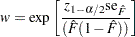 |
where  is the
  th quantile of the standard normal distribution.
Simultaneous Confidence Intervals
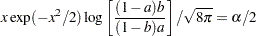
Approximate simultaneous confidence bands valid over the lifetime interval  are computed as the "Equal Precision" case of Nair (1984) and Meeker and Escobar (1998, Section 3.8) as
|
where
 |
where the factor  is the solution of
 |
The time interval over which the bands are valid depends in a complicated way on the constants  and
and  defined in Nair (1984),
  . The constants and are chosen by default so that the confidence bands are valid between the lowest and highest times corresponding to failures in the case of multiply censored data, or to the lowest and highest intervals for which probabilities are computed for arbitrarily censored data. You can optionally specify and directly with the NPINTERVALS=SIMULTANEOUS(, ) option in the PROBPLOT statement.
Copyright © SAS Institute, Inc. All Rights Reserved.