| Introduction to Bayesian Analysis Procedures |
| Summary Statistics |
Let  be a
be a  -dimensional parameter vector of interest:
  . For each
  , there are
  observations:
  .
.
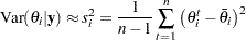
Standard Deviation
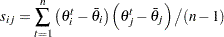
Sample standard deviation (expressed in variance term) is calculated by using the following formula:
 |
Standard Error of the Mean Estimate
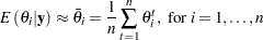
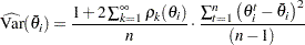
Suppose you have iid samples, the mean estimate is  , and the sample standard deviation is
  . The standard error of the estimate is
  . However, positive autocorrelation (see the section Autocorrelations for a definition) in the MCMC samples makes this an underestimate. To take account of the autocorrelation, the Bayesian procedures correct the standard error by using effective sample size (see the section Effective Sample Size).
Given an effective sample size of  , the standard error for is
  . The procedures use the following formula (expressed in variance term):
 |
The standard error of the mean is also known as the Monte Carlo standard error (MCSE). The MCSE provides a measurement of the accuracy of the posterior estimates, and small values do not necessarily indicate that you have recovered the true posterior mean.
Percentiles
Sample percentiles are calculated using Definition 5 (see Chapter 4, The UNIVARIATE Procedure (Base SAS Procedures Guide: Statistical Procedures),).
 is calculated as
Equal-Tail Credible Interval
Let  denote the marginal posterior cumulative distribution function of
  . A
. A  Bayesian equal-tail credible interval for is
  , where
  , and
, and 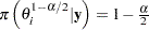 . The interval is obtained using the empirical
  th and
  th percentiles of
  .
.
Highest Posterior Density (HPD) Interval
For a definition of an HPD interval, see the section Interval Estimation. The procedures use the Chen-Shao algorithm (Chen and Shao; 1999; Chen, Shao, and Ibrahim; 2000) to estimate an empirical HPD interval of :
Sort
 to obtain the ordered values:
Compute the
credible intervals: 
for
 .
. The
HPD interval, denoted by  , is the one with the smallest interval width among all credible intervals.
Deviance Information Criterion (DIC)
The deviance information criterion (DIC) (Spiegelhalter et al.; 2002) is a model assessment tool, and it is a Bayesian alternative to Akaike’s information criterion (AIC) and the Bayesian information criterion (BIC, also known as the Schwarz criterion). The DIC uses the posterior densities, which means that it takes the prior information into account. The criterion can be applied to nonnested models and models that have non-iid data. Calculation of the DIC in MCMC is trivial—it does not require maximization over the parameter space, like the AIC and BIC. A smaller DIC indicates a better fit to the data set.
Letting be the parameters of the model, the deviance information formula is
 |
where

 : deviance
 where
 : likelihood function with the normalizing constants.
  : a standardizing term that is a function of the data alone. This term is constant with respect to the parameter and is irrelevant when you compare different models that have the same likelihood function. Since the term cancels out in DIC comparisons, its calculation is often omitted.
Note:You can think of the deviance as the difference in twice the log likelihood between the saturated,
, and fitted, , models.  : posterior mean, approximated by
 : posterior mean of the deviance, approximated by
  . The expected deviation measures how well the model fits the data.
  : deviance evaluated at
  , equal to
  . It is the deviance evaluated at your "best" posterior estimate.
  : effective number of parameters. It is the difference between the measure of fit and the deviance at the estimates:
  . This term describes the complexity of the model, and it serves as a penalization term that corrects deviance’s propensity toward models with more parameters.
Copyright © SAS Institute, Inc. All Rights Reserved.