| The LOESS Procedure |
| Sparse and Approximate Degrees of Freedom Computation |
As noted in the section Statistical Inference and Lookup Degrees of Freedom, obtaining confidence limits in loess models requires the computation of the lookup degrees of freedom. This in turn requires the computation of
 |
 |
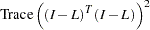 |
where  is the loess smoothing matrix (see the section Smoothing Matrix).
The work in a direct implementation of this formula grows as  , where
  is the number of observations in analysis. For large , this work dominates the time needed to fit the loess model itself. To alleviate this computational bottleneck, Cleveland and Grosse (1991) and Cleveland, Grosse, and Shyu (1992) developed approximate methods for estimating this quantity in terms of more readily computable statistics. A different approach to obtaining a computationally cheap estimate of
  has been implemented in PROC LOESS.
For large data sets with significant local structure, the loess model is often used with small values of the smoothing parameter. Recalling that the smoothing parameter defines the fraction of the data used in each local regression, this means that the loess fit at any point in regressor space depends on only a small fraction of the data. This is reflected in the smoothing matrix whose  th entry is nonzero only if the
  th and
  th observations lie in at least one common local neighborhood. Hence the smoothing matrix is a sparse matrix (has mostly zero entries) in such cases. By exploiting this sparsity, PROC LOESS now computes orders of magnitude faster than in previous implementations.
When each local neighborhood contains a large subset of the data—i.e., when the smoothing parameter is large—then it is no longer true that the smoothing matrix is sparse. However, since a point in a local neighborhood is given a local weight that decreases with its distance from the center of the neighborhood, many of the coefficients in the smoothing matrix turn out to be nonzero but with orders of magnitude smaller than that of the larger coefficients in the matrix. The approximate method for computing that has been implemented in PROC LOESS exploits these disparities in magnitudes of the elements in the smoothing matrix by setting the small elements to zero. This creates a sparse approximation of the smoothing matrix to which the fast sparse methods can be applied.
In order to decide the threshold at which elements in the smoothing matrix are set to zero, PROC LOESS samples the elements in the smoothing matrix to obtain the value of the element in a specified lower quantile in this sample. The magnitude of the element at this quantile is used as a cutoff value, and all elements in the smoothing matrix whose magnitude is less than this cutoff are set to zero for the approximate computation. By default all elements in the lower  percentile are set to zero. You can use the DFMETHOD=APPROX(QUANTILE= ) option in the MODEL statement to change this value. As you increase the value for the quantile to be zeroed, you speed up the degrees of freedom computation at the expense of increasing approximation errors. You can also use the DFMETHOD=APPROX(CUTOFF= ) option in the MODEL statement to specify the cutoff value directly.
For small data sets, the approximate computation is not needed and would be rougher than for larger data sets. Hence PROC LOESS performs the exact computation for analyses with fewer than 500 points, even if DFMETHOD=APPROX is specified in the model statement. Also, for small values of the smoothing parameter, elements in the lower specified quantile might already all be zero. In such cases the approximate method is the same as the exact method. PROC LOESS labels as approximate any statistics that depend on the approximate computation of only in the cases where the approximate computation was used and is different from the exact computation.
Copyright © 2009 by SAS Institute Inc., Cary, NC, USA. All rights reserved.