| Introduction to Statistical Modeling with SAS/STAT Software |
Least Squares
The idea of the ordinary least squares (OLS) principle is to choose parameter estimates that minimize the squared distance between the data and the model. In terms of the general, additive model,
 |
the OLS principle minimizes
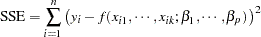 |
The least squares principle is sometimes called "nonparametric" in the sense that it does not require the distributional specification of the response or the error term, but it might be better termed "distributionally agnostic." In an additive-error model it is only required that the model errors have zero mean. For example, the specification
 |
 |
|||
 |
 |
is sufficient to derive ordinary least squares (OLS) estimators for  and
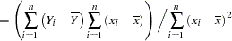
and  and to study a number of their properties. It is easy to show that the OLS estimators in this SLR model are
 |
 |
|||
 |
 |
Based on the assumption of a zero mean of the model errors, you can show that these estimators are unbiased,  ,
,  . However, without further assumptions about the distribution of the
  , you cannot derive the variability of the least squares estimators or perform statistical inferences such as hypothesis tests or confidence intervals. In addition, depending on the distribution of the , other forms of least squares estimation can be more efficient than OLS estimation.
The conditions for which ordinary least squares estimation is efficient are zero mean, homoscedastic, uncorrelated model errors. Mathematically,
 |
|
|||
 |
 |
|||
 |
 |
The second and third assumption are met if the errors have an iid distribution—that is, if they are independent and identically distributed. Note, however, that the notion of stochastic independence is stronger than that of absence of correlation. Only if the data are normally distributed does the latter implies the former.
The various other forms of the least squares principle are motivated by different extensions of these assumptions in order to find more efficient estimators.
Weighted Least Squares
The objective function in weighted least squares (WLS) estimation is
 |
where  is a weight associated with the
  th observation. A situation where WLS estimation is appropriate is when the errors are uncorrelated but not homoscedastic. If the weights for the observations are proportional to the reciprocals of the error variances,
  , then the weighted least squares estimates are best linear unbiased estimators (BLUE). Suppose that the weights are collected in the diagonal matrix
  and that the mean function has the form of a linear model. The weighted sum of squares criterion then can be written as
 |
which gives rise to the weighted normal equations
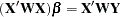 |
The resulting WLS estimator of  is
is
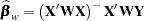 |
Iteratively Reweighted Least Squares
If the weights in a least squares problem depend on the parameters, then a change in the parameters also changes the weight structure of the model. Iteratively reweighted least squares (IRLS) estimation is an iterative technique that solves a series of weighted least squares problems, where the weights are recomputed between iterations. IRLS estimation can be used, for example, to derive maximum likelihood estimates in generalized linear models.
Generalized Least Squares
The previously discussed least squares methods have in common that the observations are assumed to be uncorrelated—that is,  , whenever
  . The weighted least squares estimation problem is a special case of a more general least squares problem, where the model errors have a general convariance matrix,
  . Suppose again that the mean function is linear, so that the model becomes
 |
The generalized least squares (GLS) principle is to minimize the generalized error sum of squares
 |
This leads to the generalized normal equations
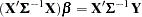 |
and the GLS estimator
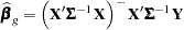 |
Obviously, WLS estimation is a special case of GLS estimation, where  —that is, the model is
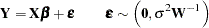 |
Copyright © 2009 by SAS Institute Inc., Cary, NC, USA. All rights reserved.