| The GLIMMIX Procedure |
Maximum Likelihood Estimation Based on Laplace Approximation
Objective Function
Let  denote the vector of fixed-effects parameters and
  the vector of covariance parameters. For Laplace estimation in the GLIMMIX procedure, includes the G-side parameters and a possible scale parameter
  , provided that the conditional distribution of the data contains such a scale parameter.
  is the vector of the G-side parameters.
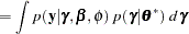
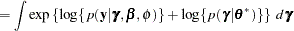
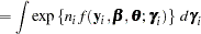
The marginal distribution of the data in a mixed model can be expressed as
 |
 |
|||
 |
 |
|||
|
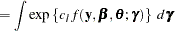 |
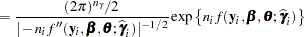
If the constant  is large, the Laplace approximation of this integral is
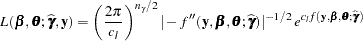 |
where  is the number of elements in
  ,
,  is the second derivative matrix
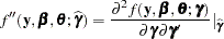 |
and  satisfies the first-order condition
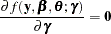 |
The objective function for Laplace parameter estimation in the GLIMMIX procedure is  . The optimization process is singly iterative, but because depends on
  and
and  , the GLIMMIX procedure solves a suboptimization problem to determine for given values of and the random-effects solution vector that maximizes
  .
.
When you have longitudinal or clustered data with  independent subjects or clusters, the vector of observations can be written as
  , where
  is an
is an  vector of observations for subject (cluster)
  (
( ). In this case, assuming conditional independence such that
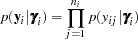 |
the marginal distribution of the data can be expressed as
 |
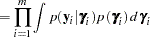 |
|||
|
 |
where
 |
 |
|||
|
 |
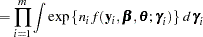
When the number of observations within a cluster,  , is large, the Laplace approximation to the th individual’s marginal probability density function is
 |
 |
|||
|
 |
where  is the common dimension of the random effects,
  . In this case, provided that the constant
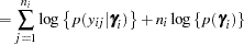
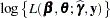
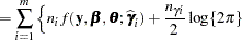
  is large, the Laplace approximation to the marginal log likelihood is
 |
 |
|||
|
 |
which serves as the objective function for the METHOD=LAPLACE estimator in PROC GLIMMIX.
The Laplace approximation implemented in the GLIMMIX procedure differs from that in Wolfinger (1993) and Pinheiro and Bates (1995) in important respects. Wolfinger (1993) assumed a flat prior for and expanded the integrand around and , leaving only the covariance parameters for the overall optimization. The "fixed" effects and the random effects are determined in a suboptimization that takes the form of a linear mixed model step with pseudo-data. The GLIMMIX procedure involves only the random effects vector in the suboptimization. Pinheiro and Bates (1995) and Wolfinger (1993) consider a modified Laplace approximation that replaces the second derivative  with an (approximate) expected value, akin to scoring. The GLIMMIX procedure does not use an approximation to . The METHOD=RSPL estimates in PROC GLIMMIX are equivalent to the estimates obtained with the modified Laplace approximation in Wolfinger (1993). The objective functions of METHOD=RSPL and Wolfinger (1993) differ in a constant that depends on the number of parameters.
Asymptotic Properties and the Importance of Subjects
Suppose that the GLIMMIX procedure processes your data by subjects (see the section Processing by Subjects) and let denote the number of observations per subject,  . Arguments in Vonesh (1996) show that the maximum likelihood estimator based on the Laplace approximation is a consistent estimator to order
  . In other words, as the number of subjects and the number of observations per subject grows, the small-sample bias of the Laplace estimator disappears. Note that the term involving the number of subjects in this maximum relates to standard asymptotic theory, and the term involving the number of observations per subject relates to the accuracy of the Laplace approximation (Vonesh 1996). In the case where random effects enter the model linearly, the Laplace approximation is exact and the requirement that
  can be dropped.
If your model is not processed by subjects but is equivalent to a subject model, the asymptotics with respect to  still apply, because the Hessian matrix of the suboptimization for breaks into separate blocks. For example, the following two models are equivalent with respect to and , although only for the first model does PROC GLIMMIX process the data explicitly by subjects:
   proc glimmix method=laplace;
      class sub A;
      model y = A;
      random intercept / subject=sub;
   run;
   proc glimmix method=laplace;
      class sub A;
      model y = A;
      random sub;
   run;
The same holds, for example, for models with independent nested random effects. The following two models are equivalent, and you can derive asymptotic properties related to and  from the model in the first run:
   proc glimmix method=laplace;
      class A B block;
      model y = A B A*B;
      random intercept A / subject=block;
   run;

   proc glimmix method=laplace;
      class A B block;
      model y = A B A*B;
      random block a*block;
   run;
The Laplace approximation requires that the dimension of the integral does not increase with the size of the sample. Otherwise the error of the likelihood approximation does not diminish with . This is the case, for example, with exchangeable arrays (Shun and McCullagh 1995), crossed random effects (Shun 1997), and correlated random effects of arbitrary dimension (Raudenbush, Yang, and Yosef 2000). Results in Shun (1997), for example, show that even in this case the standard Laplace approximation has smaller bias than pseudo-likelihood estimates.
Copyright © 2009 by SAS Institute Inc., Cary, NC, USA. All rights reserved.