Tests for Normality

Distribution Analyses

Tests for Normality

SAS/INSIGHT software provides tests for the null hypothesis that the input data values are a random sample from a normal distribution. These test statistics include the Shapiro-Wilk statistic (W) and statistics based on the empirical distribution function: the Kolmogorov-Smirnov, Cramer-von Mises, and Anderson-Darling statistics.

The Shapiro-Wilk statistic is the ratio of the best estimator of the variance (based on the square of a linear combination of the order statistics) to the usual corrected sum of squares estimator of the variance. W must be greater than zero and less than or equal to one, with small values of W leading to rejection of the null hypothesis of normality. Note that the distribution of W is highly skewed. Seemingly large values of W (such as 0.90) may be considered small and lead to the rejection of the null hypothesis.

The W statistic is computed when the sample size is less than or equal to 2000. When the sample size is greater than three, the coefficients for computing the linear combination of the order statistics are approximated by the method of Royston (1992).

With a sample size of three, the probability distribution of W is known and is used to determine the significance level. When the sample size is greater than three, simulation results are used to obtain the approximate normalizing transformation (Royston 1992)

$Z_{n} = \{ ( -\log( \gamma - \log(1-W_{n}) ) - \mu) / \sigma & {if 4 \le n \le 11} \ ( \log( 1-W_{n}) - \mu ) / \sigma & {if 12 \le n \le 2000} \ .$

where $\gamma$ , $\mu$ , and $\sigma$ are functions of n, obtained from simulation results, and Z_n is a standard normal variate with large values indicating departure from normality.

The Kolmogorov statistic assesses the discrepancy between the empirical distribution and the estimated hypothesized distribution. For a test of normality, the hypothesized distribution is a normal distribution function with parameters $\mu$ and $\sigma$ estimated by the sample mean and standard deviation. The probability of a larger test statistic is obtained by linear interpolation within the range of simulated critical values given by Stephens (1974).

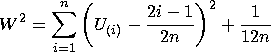
The Cramer-von Mises statistic ( W²) is defined as

$W^2 = n \int_{-\infty}^{\infty}{(F_{n}(x) - F(x))^2 dF(x) }$

and it is computed as

$W^2 = \sum_{i=1}^n( U_{(i)} - \frac{2i-1}{2n} )^2 + \frac{1}{12n }$

where U_(i) = F(y_(i)) is the cumulative distribution function value at y_(i), the ith ordered value. The probability of a larger test statistic is obtained by linear interpolation within the range of simulated critical values given by Stephens (1974).

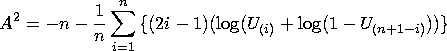
The Anderson-Darling statistic ( A²) is defined as

$A^2 = n \int_{-\infty}^{\infty}{(F_{n}(x) - F(x))^2 \{F(x) (1-F(x))\}^{-1} dF(x) }$

and it is computed as

$A^2 = -n - \frac{1}n \sum_{i=1}^n{\{(2i-1) ( \log(U_{(i)} + \log(1-U_{(n+1-i)}) ) \} }$

The probability of a larger test statistic is obtained by linear interpolation within the range of simulated critical values in D'Agostino and Stephens (1986).

A Tests for Normality table includes the Shapiro-Wilk, Kolmogorov, Cramer-von Mises, and Anderson-Darling test statistics, with their corresponding p-values, as shown in Figure 38.14.

Top of Page