The OPTEX Procedure

Note: See Adding Space-filling Points to a Design in the SAS/QC Sample Library.

Suppose you want a 15-run experiment for three mixture factors x1, x2, and x3; furthermore, suppose that x3 cannot account for any more than 75% of the mixture. The vertices and generalized edge centroids of the region defined by these constraints make up a good candidate set to use with the OPTEX procedure for finding a D-optimal design for such an experiment. However, information-based criteria such as D- and A-efficiency tend to push the design to the edges of the candidate space, leaving large portions of the interior relatively uncovered. For this reason, it is often a good idea to augment a D-optimal design with some points chosen according to U-optimality, which seeks to cover the candidate region as well as possible.

The following statements create a candidate data set containing 216 points in the region defined by the given constraints and on the factors:

data a;
   do x1 = 0 to 100 by 5;                       
      do x3 = 0 to 100 by 5;
         x2 = 100 - x1 - x3;
         if (0<= x2 <= 75) then output;
      end; 
   end;
run;
data a; set a;
   x1 = x1 / 100;
   x2 = x2 / 100;
   x3 = x3 / 100;
run;

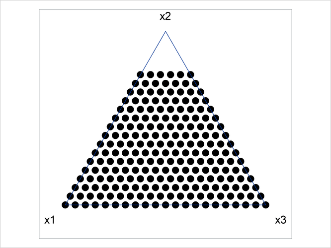
The constraint that the factor levels sum to 1 means that the candidate points all lie on a plane. Thus, the values of all three variables can be displayed in a two-dimensional "mixture plot," as shown in Output 14.10.1.

You can use the OPTEX procedure to select 10 points from the mentioned candidate points optimal for estimating a second-order model in the mixture factors.

proc optex data=a seed=60868 nocode;
   model x1|x2|x3@2 / noint;     
   generate n=10;
   output out=b;             
run;

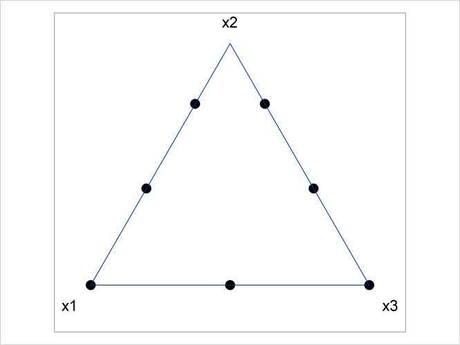
The resulting points are plotted in Output 14.10.2. There are only seven unique points, indicating that the D-optimal design replicates some chosen candidate points.

The D-optimal design leaves a large "hole" in the feasible region. The following statements "fill in the hole" in the optimal design saved in B by augmenting it with points chosen from the candidate data set a to optimize the U-criterion:

proc optex data=a seed=4321 nocode;
   model x1 x2 x3 / noint;          
   generate n=15 augment=b criterion=u;
   output out=c;
run;

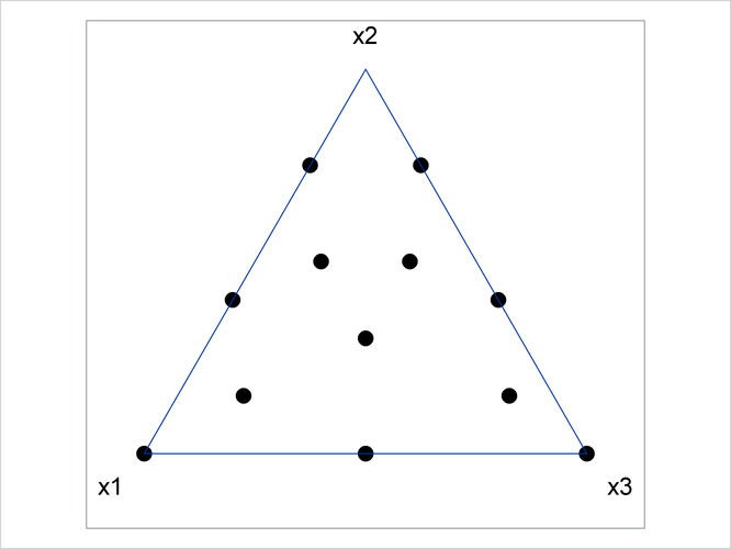
The resulting points are shown in Output 14.10.3. The U-optimal design fills in the candidate region in much the same way that you might construct the design by visually assigning points. That is, the general approach that uses the OPTEX procedure agrees with visual intuition for this small problem. This indicates that the general approach will yield an appropriate design for higher-dimensional problems that cannot be visualized.