The CAPABILITY Procedure
Summary of Theoretical Distributions
You can use the PPPLOT statement to request P-P plots based on the theoretical distributions summarized in the following table:
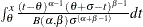
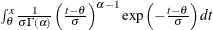
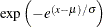
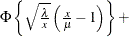
Table 5.56: Distributions and Parameters
|
Parameters |
||||||
|---|---|---|---|---|---|---|
|
Family |
Distribution Function |
Range |
Location |
Scale |
Shape |
|
|
Beta |
|
|
|
|
|
|
|
Exponential |
|
|
|
|
||
|
Gamma |
|
|
|
|
|
|
|
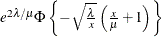
Gumbel |
|
all x |
|
|
||
|
Inverse Gaussian |
|
x > 0 |
|
|
||
|
|
||||||
|
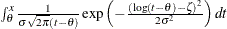
Lognormal |
|
|
|
|
|
|
|
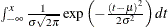
Normal |
|
all x |
|
|
||
|
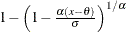
Generalized Pareto |
|
all x |
|
|
|
|
|
Power Function |
|
|
|
|
|
|
|
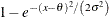
Rayleigh |
|
|
|
|
||
|
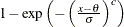
Weibull |
|
|
|
|
c |
|


You can request these distributions with the BETA , EXPONENTIAL , GAMMA , GUMBEL , IGAUSS , NORMAL , LOGNORMAL , PARETO , POWER , RAYLEIGH , and WEIBULL options, respectively. If you do not specify a distribution option, a normal P-P plot is created.
To create a P-P plot, you must provide all of the parameters for the theoretical distribution. If you do not specify parameters, then default values or estimates are substituted, as summarized by the following table:
Table 5.57: Defaults for Parameters
|
Family |
Default Values |
Estimated Values |
|---|---|---|
|
Beta |
|
maximum likelihood estimates for |
|
Exponential |
|
maximum likelihood estimate for |
|
Gamma |
|
maximum likelihood estimates for |
|
Gumbel |
None |
maximum likelihood estimates for |
|
Inverse Gaussian |
None |
sample estimate for |
|
Lognormal |
|
maximum likelihood estimates for |
|
Normal |
None |
sample estimates for |
|
Generalized Pareto |
|
maximum likelihood estimates for |
|
Power Function |
|
maximum likelihood estimate for |
|
Rayleigh |
|
maximum likelihood estimate for |
|
Weibull |
|
maximum likelihood estimates for |

