The SHEWHART Procedure
The following example[53] is adapted from an application in aircraft component manufacturing. A metal extrusion process is used to make three slightly different models of the same component. The three product types (labeled M1, M2, and M3) are produced in small quantities because the process is expensive and time-consuming.
Figure 17.205 shows the structure of a SAS data set named Old, which contains the diameter measurements for various short runs. Samples 1 to 30 are to be used to estimate the process
standard deviation ![]() for the differences from nominal.
for the differences from nominal.
Figure 17.205: Diameter Measurements in the Data Set Old
| Sample | Prodtype | Diameter |
|---|---|---|
| 1 | M3 | 13.99 |
| 2 | M3 | 14.69 |
| 3 | M3 | 13.86 |
| 4 | M3 | 14.32 |
| 5 | M3 | 13.23 |
| 6 | M1 | 17.55 |
| 7 | M1 | 14.26 |
| 8 | M1 | 14.62 |
| 9 | M1 | 12.97 |
| 10 | M2 | 16.18 |
| 11 | M2 | 15.29 |
| 12 | M2 | 16.20 |
| 13 | M3 | 13.89 |
| 14 | M3 | 12.71 |
| 15 | M3 | 14.32 |
| 16 | M3 | 15.35 |
| 17 | M2 | 15.08 |
| 18 | M2 | 14.72 |
| 19 | M2 | 14.79 |
| 20 | M2 | 15.27 |
| 21 | M2 | 15.95 |
| 22 | M1 | 14.78 |
| 23 | M1 | 15.19 |
| 24 | M1 | 15.41 |
| 25 | M1 | 16.26 |
| 26 | M3 | 16.68 |
| 27 | M3 | 15.60 |
| 28 | M3 | 14.86 |
| 29 | M3 | 16.67 |
| 30 | M3 | 14.35 |
In short run applications involving many product types, it is common practice to maintain a database for the nominal values
for the product types. Here, the nominal values are saved in a SAS data set named Nomval, which is listed in Figure 17.206.
To compute the differences from nominal, you must merge the data with the nominal values. You can do this with the following
SAS statements. Note that an IN= variable is used in the MERGE statement to allow for the fact that Nomval includes nominal values for product types that are not represented in Old. Figure 17.207 lists the merged data set Old.
proc sort data=Old;
   by Prodtype;
run;

data Old;
   format Diff 5.2 ;
   merge Nomval Old(in = a);
      by Prodtype;
   if a;
   Diff = Diameter - Nominal;
run;

proc sort data=Old;
   by Sample;
run;
Figure 17.207: Data Merged with Nominal Values
| Sample | Prodtype | Diameter | Nominal | Diff |
|---|---|---|---|---|
| 1 | M3 | 13.99 | 14.8 | -0.81 |
| 2 | M3 | 14.69 | 14.8 | -0.11 |
| 3 | M3 | 13.86 | 14.8 | -0.94 |
| 4 | M3 | 14.32 | 14.8 | -0.48 |
| 5 | M3 | 13.23 | 14.8 | -1.57 |
| 6 | M1 | 17.55 | 15.0 | 2.55 |
| 7 | M1 | 14.26 | 15.0 | -0.74 |
| 8 | M1 | 14.62 | 15.0 | -0.38 |
| 9 | M1 | 12.97 | 15.0 | -2.03 |
| 10 | M2 | 16.18 | 15.5 | 0.68 |
| 11 | M2 | 15.29 | 15.5 | -0.21 |
| 12 | M2 | 16.20 | 15.5 | 0.70 |
| 13 | M3 | 13.89 | 14.8 | -0.91 |
| 14 | M3 | 12.71 | 14.8 | -2.09 |
| 15 | M3 | 14.32 | 14.8 | -0.48 |
| 16 | M3 | 15.35 | 14.8 | 0.55 |
| 17 | M2 | 15.08 | 15.5 | -0.42 |
| 18 | M2 | 14.72 | 15.5 | -0.78 |
| 19 | M2 | 14.79 | 15.5 | -0.71 |
| 20 | M2 | 15.27 | 15.5 | -0.23 |
| 21 | M2 | 15.95 | 15.5 | 0.45 |
| 22 | M1 | 14.78 | 15.0 | -0.22 |
| 23 | M1 | 15.19 | 15.0 | 0.19 |
| 24 | M1 | 15.41 | 15.0 | 0.41 |
| 25 | M1 | 16.26 | 15.0 | 1.26 |
| 26 | M3 | 16.68 | 14.8 | 1.88 |
| 27 | M3 | 15.60 | 14.8 | 0.80 |
| 28 | M3 | 14.86 | 14.8 | 0.06 |
| 29 | M3 | 16.67 | 14.8 | 1.87 |
| 30 | M3 | 14.35 | 14.8 | -0.45 |
Assume that the variability in the process is constant across product types. To estimate the common process standard deviation
![]() , you first estimate
, you first estimate ![]() for each product type based on the average of the moving ranges of the differences from nominal. You can do this in several
steps, the first of which is to sort the data and compute the average moving range with the SHEWHART procedure.
for each product type based on the average of the moving ranges of the differences from nominal. You can do this in several
steps, the first of which is to sort the data and compute the average moving range with the SHEWHART procedure.
proc sort data=Old;
   by Prodtype;
run;

proc shewhart data=Old;
   irchart Diff*Sample /
      nochart
      outlimits=Baselim;
   by Prodtype;
run;
The purpose of this procedure step is simply to save the average moving range for each product type in the OUTLIMITS= data
set Baselim, which is listed in Figure 17.208 (note that Prodtype is specified as a BY variable).
Figure 17.208: Values of ![]() by Product Type
by Product Type
| Control Limits By Product Type |
| Prodtype | _VAR_ | _SUBGRP_ | _TYPE_ | _LIMITN_ | _ALPHA_ | _SIGMAS_ | _LCLI_ | _MEAN_ | _UCLI_ | _LCLR_ | _R_ | _UCLR_ | _STDDEV_ |
|---|---|---|---|---|---|---|---|---|---|---|---|---|---|
| M1 | Diff | Sample | ESTIMATE | 2 | .002699796 | 3 | -3.13258 | 0.13000 | 3.39258 | 0 | 1.22714 | 4.00850 | 1.08753 |
| M2 | Diff | Sample | ESTIMATE | 2 | .002699796 | 3 | -1.77795 | -0.06500 | 1.64795 | 0 | 0.64429 | 2.10458 | 0.57098 |
| M3 | Diff | Sample | ESTIMATE | 2 | .002699796 | 3 | -3.22641 | -0.19143 | 2.84356 | 0 | 1.14154 | 3.72887 | 1.01166 |
To obtain a combined estimate of ![]() , you can use the MEANS procedure to average the average ranges in
, you can use the MEANS procedure to average the average ranges in Baselim and then divide by the unbiasing constant ![]() .
.
proc means data=Baselim noprint;
   var _r_;
   output out=Difflim (keep=_r_) mean=_r_;
run;

data Difflim;
   set Difflim;
   drop _r_;
   length _var_ _subgrp_ $ 8;
   _var_    = 'Diff';
   _subgrp_ = 'Sample';
   _mean_   = 0.0;
   _stddev_ = _r_ / d2(2);
   _limitn_ = 2;
   _sigmas_ = 3;
run;
The data set Difflim is structured for subsequent use by the SHEWHART procedure as an input LIMITS= data set. The variables in a LIMITS= data
set provide pre-computed control limits or—as in this case—the parameters from which control limits are to be computed. These
variables have reserved names that begin and end with the underscore character. Here, the variable _STDDEV_ saves the estimate of ![]() , and the variable
, and the variable _MEAN_ saves the mean of the differences from nominal. Recall that this mean is zero, since the nominal values are assumed to represent
the process mean for each product type. The identifier variables _VAR_ and _SUBGRP_ record the names of the process and subgroup variables (these variables are critical in applications involving many product
types). The variable _LIMITN_ is assigned a value of 2 to specify moving ranges of two consecutive measurements, and the variable _SIGMAS_ is assigned a value of 3 to specify ![]() limits. The data set
limits. The data set Difflim is listed in Figure 17.209.
Now that the control limit parameters are saved in Difflim, diameters for an additional 30 parts (samples 31 to 60) are measured and saved in a SAS data set named New. You can construct short run control charts for this data by merging the measurements in New with the corresponding nominal values in Nomval, computing the differences from nominal, and then constructing the short run individual measurements and moving range charts.
proc sort data=new;
   by Prodtype;
run;

data new;
   format Diff 5.2 ;
   merge Nomval new(in = a);
      by Prodtype;
   if a;
   Diff = Diameter - Nominal;
   label Sample   = 'Sample Number'
         Prodtype = 'Model';
run;

proc sort data=new;
   by Sample;
run;
ods graphics off;
symbol1 v=dot    c=blue  h=3.0 pct;
symbol2 v=plus   c=red   h=3.0 pct;
symbol3 v=circle c=green h=3.0 pct;
title 'Chart for Difference from Nominal';
proc shewhart data=new limits=Difflim;
   irchart Diff*Sample=Prodtype / split    = '/';
   label Diff = 'Difference/Moving Range';
run;
The chart is displayed in Figure 17.210. Note that the product types are identified with symbol markers as requested by specifying Prodtype as a symbol-variable.
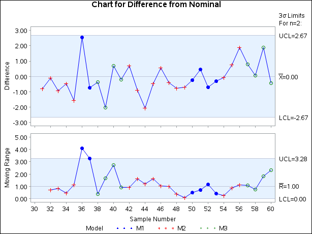
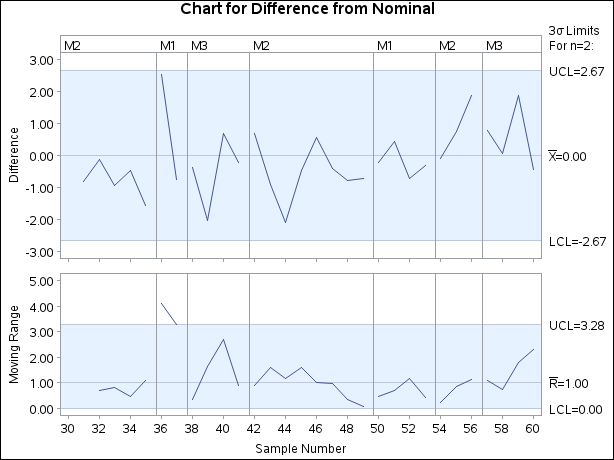
You can also identify the product types with a legend by specifying Prodtype as a _PHASE_ variable.
symbol h=3.0 pct;
title 'Chart for Difference from Nominal';
proc shewhart data=new (rename=(Prodtype=_phase_)) limits=Difflim;
   irchart Diff*Sample /
      readphases = all
      phaseref
      phasebreak
      phaselegend
      split      = '/';
   label Diff = 'Difference/Moving Range';
run;
The display is shown in Figure 17.211. Note that the PHASEBREAK option is used to suppress the connection of adjacent points in different phases (product types).
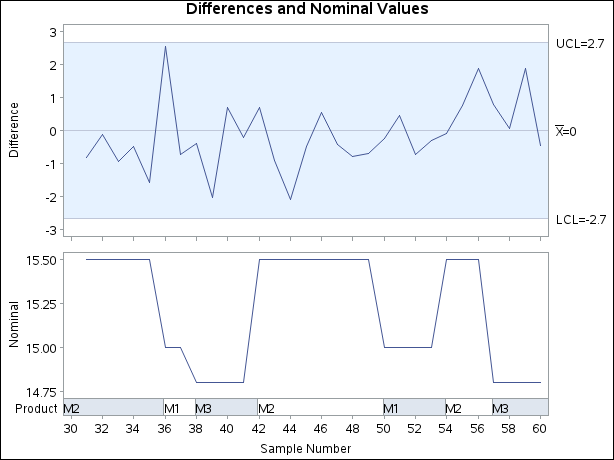
In some applications, it may be useful to replace the moving range chart with a plot of the nominal values. You can do this
with the TRENDVAR= option in the XCHART statement[54] provided that you reset the value of _LIMITN_ to 1 to specify a subgroup sample of size one.
data Difflim;
   set Difflim;
   _var_    = 'Diameter';
   _limitn_ = 1;
run;
title 'Differences and Nominal Values';
proc shewhart data=new limits=Difflim;
   xchart Diameter*Sample (Prodtype) /
      nolimitslegend
      nolegend
      split         = '/'
      blockpos      = 3
      blocklabtype  = scaled
      blocklabelpos = left
      xsymbol       = xbar
      trendvar      = Nominal;
   label Diameter   = 'Difference/Nominal'
         Prodtype   = 'Product';
run;
The display is shown in Figure 17.212. Note that you identify the product types by specifying Prodtype as a block variable enclosed in parentheses after the subgroup variable Sample. The BLOCKLABTYPE= option specifies that values of the block variable are to be scaled (if necessary) to fit the space available
in the block legend. The BLOCKLABELPOS= option specifies that the label of the block variable is to be displayed to the left
of the block legend.