The SHEWHART Procedure

Autocorrelation in Process Data

Subsections:

Note: See Autocorrelation in Process Data in the SAS/QC Sample Library.

Autocorrelation has long been recognized as a natural phenomenon in process industries, where parameters such as temperature and pressure vary slowly relative to the rate at which they are measured. Only in recent years has autocorrelation become an issue in SPC applications, particularly in parts industries, where autocorrelation is viewed as a problem that can undermine the interpretation of Shewhart charts. One reason for this concern is that, as automated data collection becomes prevalent in parts industries, processes are sampled more frequently and it is possible to recognize autocorrelation that was previously undetected. Another reason, noted by Box and Kramer (1992), is that the distinction between parts and process industries is becoming blurred in areas such as computer chip manufacturing. For two other discussions of this issue, refer to Schneider and Pruett (1994) and Woodall (1993).

The standard Shewhart analysis of individual measurements assumes that the process operates with a constant mean $\mu$ , and that $x_{t}$ (the measurement at time t) can be represented as $x_{t} = \mu + \epsilon _{t}$ , where $\epsilon _{t}$ is a random displacement or error from the process mean $\mu$ . Typically, the errors are assumed to be statistically independent in the derivation of the control limits displayed at three standard deviations above and below the central line, which represents an estimate for $\mu$ .

When Shewhart charts are constructed from autocorrelated measurements, the result can be too many false signals, making the control limits seem too tight. This situation is illustrated in Figure 17.191, which displays an individual measurement and moving range chart for 100 observations of a chemical process.

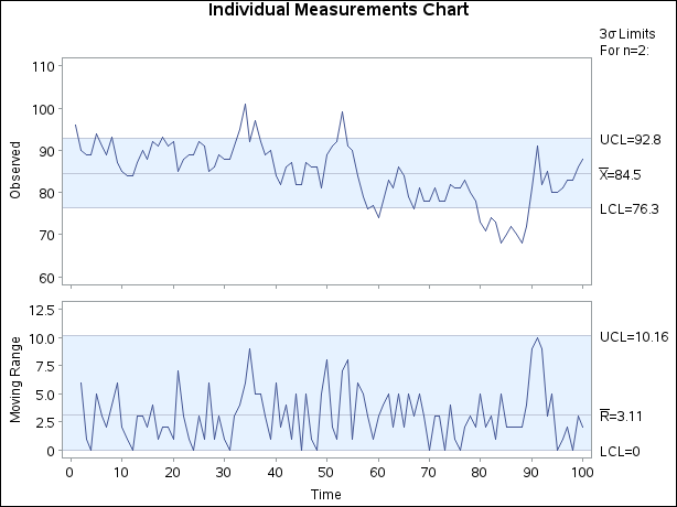
Figure 17.191: Conventional Shewhart Chart

The measurements are saved in a SAS data set named Chemical.^[45] The chart in Figure 17.191 is created with the following statements:

symbol h=2.0 pct;
title 'Individual Measurements Chart';
proc shewhart data=Chemical;
   irchart xt*t / npanelpos = 100
                  split     = '/';
   label xt = 'Observed/Moving Range'
          t = 'Time';
run;

^[45]The measurements are patterned after the values plotted in Figure 1 of Montgomery and Mastrangelo (1991).