The OPTEX Procedure
An optimality criterion is a single number that summarizes how good a design is, and it is maximized or minimized by an optimal design. This section discusses in detail the optimality criteria available in the OPTEX procedure.
Two general types of criteria are available: information-based criteria and distance-based criteria.
The information-based criteria that are directly available are D- and A-optimality; they are both related to the information
matrix ![]() for the design. This matrix is important because it is proportional to the inverse of the variance-covariance matrix for
the least squares estimates of the linear parameters of the model. Roughly, a good design should "minimize" the variance
for the design. This matrix is important because it is proportional to the inverse of the variance-covariance matrix for
the least squares estimates of the linear parameters of the model. Roughly, a good design should "minimize" the variance ![]() , which is the same as "maximizing" the information
, which is the same as "maximizing" the information ![]() . D- and A-efficiency are different ways of saying how large
. D- and A-efficiency are different ways of saying how large ![]() or
or ![]() are.
are.
For the distance-based criteria, the candidates are viewed as comprising a point cloud in p-dimensional Euclidean space, where p is the number of terms in the model. The goal is to choose a subset of this cloud that "covers" the whole cloud as uniformly as possible (in the case of U-optimality) or that is as broadly "spread" as possible (in the case of S-optimality). These ideas of coverage and spread are defined in detail in the section Distance-Based Criteria. The distance-based criteria thus correspond to the intuitive idea of filling the candidate space as well as possible.
The rest of this section discusses different optimality criterion in detail.
D-optimality is based on the determinant of the information matrix for the design, which is the same as the reciprocal of the determinant of the variance-covariance matrix for the least squares estimates of the linear parameters of the model.
The determinant is thus a general measure of the size of ![]() . D-optimality is the most commonly used criterion for generating optimal designs. This explains why it is the default criterion
for the OPTEX procedure.
. D-optimality is the most commonly used criterion for generating optimal designs. This explains why it is the default criterion
for the OPTEX procedure.
The D-optimality criterion has the following characteristics:
-
D-optimality is the most computationally efficient criterion to optimize for the low-rank update algorithms of the OPTEX procedure, since each update depends only on the variance of prediction for the current design; see the section Useful Matrix Formulas.
-
 is inversely proportional to the size of a
  confidence ellipsoid for the least squares estimates of the linear parameters of the model.
-
 is equal to the geometric mean of the eigenvalues of
  .
.
-
The D-optimal design is invariant to nonsingular recoding of the design matrix.

A-optimality is based on the sum of the variances of the estimated parameters for the model, which is the same as the sum
of the diagonal elements, or trace, of ![]() . Like the determinant, the A-optimality criterion is a general measure of the size of
. Like the determinant, the A-optimality criterion is a general measure of the size of ![]() . A-optimality is less commonly used than D-optimality as a criterion for computer optimal design. This is partly because
it is more computationally difficult to update; see the section Useful Matrix Formulas. Also, A-optimality is not invariant to nonsingular recoding of the design matrix; different designs will be optimal with different codings.
. A-optimality is less commonly used than D-optimality as a criterion for computer optimal design. This is partly because
it is more computationally difficult to update; see the section Useful Matrix Formulas. Also, A-optimality is not invariant to nonsingular recoding of the design matrix; different designs will be optimal with different codings.
Both G-efficiency and the average prediction variance are well-known criteria for optimal design. Both are based on the variance
of prediction of the candidate points, which is proportional to ![]() . As this formula shows, these two criteria are also related to the information matrix
. As this formula shows, these two criteria are also related to the information matrix ![]() . Minimizing the average prediction variance has also been called I-optimality, the "I" denoting integration over the candidate space.
. Minimizing the average prediction variance has also been called I-optimality, the "I" denoting integration over the candidate space.
It is possible to apply the search techniques available in the OPTEX procedure to these two criteria, but this turns out to be a poor way to find G- and I-optimal designs. One reason for this is that there are no efficient low-rank update rules (see the section Useful Matrix Formulas, so that the searches can take a very long time. More seriously, for G-optimality such a search often does not converge on a design with good G-efficiency. G-efficiency is simply too "rough" a criterion to be optimized by the relatively short steps of the search algorithms available in the OPTEX procedure.
However, the OPTEX procedure does offer an approach for finding G-efficient designs. Begin by searching for designs according to the default D-optimality criterion. Then, from the various designs found on the different tries, you can save the one that has the best G-efficiency by specifying the NUMBER=GBEST option in the OUTPUT statement. Since D- and G-efficiency are highly correlated over the space of all designs, this method usually results in adequately G-efficient designs, especially when the number of tries is large (see Nguyen and Piepel (2005)). See the ITER= option for details on specifying the number of tries.
To find I-optimal designs, note that if the design is orthogonally coded then I-optimality is equivalent to the A-optimality,
since the sum of the prediction variances of all points ![]() in the candidate space
in the candidate space ![]() is
is
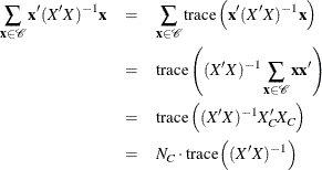
where ![]() is the number of candidate points and
is the number of candidate points and ![]() is the design matrix for the candidate points. Thus, you can use the option CODING=ORTH in the PROC OPTEX statement together
with the option CRITERION=A in the GENERATE statement to search for I-optimal designs.
is the design matrix for the candidate points. Thus, you can use the option CODING=ORTH in the PROC OPTEX statement together
with the option CRITERION=A in the GENERATE statement to search for I-optimal designs.
Note that both G- and I-optimality are invariant to nonsingular recoding of the design matrix, since the coding does not affect how well a point is predicted.
The distance-based criteria are based on the distance ![]() from a point
from a point ![]() in the p-dimensional Euclidean space
in the p-dimensional Euclidean space ![]() to a set
to a set ![]() . This distance is defined as follows:
. This distance is defined as follows:
where ![]() is the usual p-dimensional Euclidean distance,
is the usual p-dimensional Euclidean distance,
U-optimality seeks to minimize the sum of the distances from each candidate point to the design.
where ![]() is the set of candidate points and
is the set of candidate points and ![]() is the set of design points. You can visualize the U criterion by associating with any design point those candidates to which
it is closest. Thus, the design defines a clustering of the candidate set, and indeed cluster analysis has been used in this context. Johnson, Moore, and Ylvisaker (1990) consider a similar measure of design efficiency, but over infinite rather than finite candidate spaces. Computationally,
the U-optimality criterion can be very difficult to optimize, especially if the matrix of all pairwise distances between candidate points does not fit in memory.
In this case, the OPTEX procedure recomputes each distance as needed. When searching for a U-optimal design, you should start
with a small version of the problem to get an idea of the computing resources required.
is the set of design points. You can visualize the U criterion by associating with any design point those candidates to which
it is closest. Thus, the design defines a clustering of the candidate set, and indeed cluster analysis has been used in this context. Johnson, Moore, and Ylvisaker (1990) consider a similar measure of design efficiency, but over infinite rather than finite candidate spaces. Computationally,
the U-optimality criterion can be very difficult to optimize, especially if the matrix of all pairwise distances between candidate points does not fit in memory.
In this case, the OPTEX procedure recomputes each distance as needed. When searching for a U-optimal design, you should start
with a small version of the problem to get an idea of the computing resources required.
S-optimality seeks to maximize the harmonic mean distance from each design point to all the other points in the design.
For an S-optimal design, the distances ![]() are large, so the points are as spread out as possible. Since the S-optimality criterion depends only on the distances between
design points, it is usually computationally easier to compute and optimize than the U-optimality criterion, which depends
on the distances between all pairs of candidate points.
are large, so the points are as spread out as possible. Since the S-optimality criterion depends only on the distances between
design points, it is usually computationally easier to compute and optimize than the U-optimality criterion, which depends
on the distances between all pairs of candidate points.