The OUTLIMITS= option saves the control limits from the chart in Figure 17.215 in a SAS data set named DELAYLIM, which is listed in Figure 17.216.
Figure 17.216: Control Limits for Standard Chart from the Data Set Calls
| _VAR_ | _SUBGRP_ | _TYPE_ | _LIMITN_ | _ALPHA_ | _SIGMAS_ | _LCLI_ | _MEAN_ | _UCLI_ | _STDDEV_ |
|---|---|---|---|---|---|---|---|---|---|
| Time | Recnum | ESTIMATE | 2 | .002699796 | 3 | 1.77008 | 2.91038 | 4.05068 | 0.38010 |
The control limits can be replaced with the corresponding percentiles from a fitted lognormal distribution. The equation for the lognormal density function is
where ![]() denotes the shape parameter and
denotes the shape parameter and ![]() denotes the scale parameter.
denotes the scale parameter.
The following statements use the CAPABILITY procedure to fit a lognormal model and superimpose the fitted density on a histogram of the data, shown in Figure 17.217:
title 'Lognormal Fit for Delay Distribution';
proc capability data=Calls noprint;
   histogram Time /
      lognormal(threshold=2.3 w=2)
      outfit = Lnfit
      nolegend ;
   inset n = 'Number of Calls'
      lognormal( sigma = 'Shape' (4.2)
                 zeta  = 'Scale' (5.2)
                 theta ) / pos    = ne;
   label Time  = 'Answering Delay (minutes)';
run;
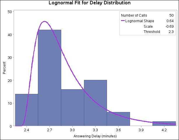
Parameters of the fitted distribution and results of goodness-of-fit tests are saved in the data set LNFIT, which is listed in Figure 17.218. The large p-values for the goodness-of-fit tests are evidence that the lognormal model provides a good fit.
Figure 17.218: Parameters of Fitted Lognormal Model in the Data Set LNFIT
| _VAR_ | _CURVE_ | _LOCATN_ | _SCALE_ | _SHAPE1_ | _MIDPTN_ | _ADASQ_ | _ADP_ | _CVMWSQ_ | _CVMP_ | _KSD_ | _KSP_ |
|---|---|---|---|---|---|---|---|---|---|---|---|
| Time | LNORMAL | 2.3 | -0.68910 | 0.64110 | 4.2 | 0.34854 | 0.47465 | 0.058737 | 0.40952 | 0.092223 | 0.15 |
The following statements replace the control limits in DELAYLIM with limits computed from percentiles of the fitted lognormal
model. The 100![]() th percentile of the lognormal distribution is
th percentile of the lognormal distribution is ![]() , where
, where ![]() denotes the inverse standard normal cumulative distribution function. The SHEWHART procedure constructs an X chart with the modified limits, displayed in Figure 17.219.
denotes the inverse standard normal cumulative distribution function. The SHEWHART procedure constructs an X chart with the modified limits, displayed in Figure 17.219.
data delaylim;
   merge delaylim Lnfit;
   drop _sigmas_ ;
   _lcli_ = _locatn_ + exp(_scale_+probit(0.5*_alpha_)*_shape1_);
   _ucli_ = _locatn_ + exp(_scale_+probit(1-.5*_alpha_)*_shape1_);
   _mean_ = _locatn_ + exp(_scale_+0.5*_shape1_*_shape1_);
run;
title 'Lognormal Control Limits for Delays';
proc shewhart data=Calls limits=delaylim;
   irchart Time*Recnum /
      rtmplot   = schematic
      nochart2 ;
   label Recnum = 'Record Number'
         Time   = 'Delay in minutes' ;
run;
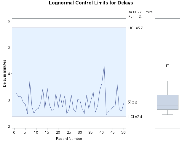
Clearly the process is in control, and the control limits (particularly the lower limit) are appropriate for the data. The
particular probability level ![]() associated with these limits is somewhat immaterial, and other values of
associated with these limits is somewhat immaterial, and other values of ![]() such as 0.001 or 0.01 could be specified with the ALPHA= option in the original IRCHART statement.
such as 0.001 or 0.01 could be specified with the ALPHA= option in the original IRCHART statement.