: BAYESACT Call

BAYESACT Call

computes posterior probabilities that observations are contaminated with a larger variance.

Syntax

CALL BAYESACT $\text{[math]}$

where

$\text{[math]}$	is the contamination coefficient, where $\text{[math]}$ .
$\text{[math]}$	is an independent estimate of $\text{[math]}$ , where $\text{[math]}$ .
$\text{[math]}$	is the number of degrees of freedom for $\text{[math]}$ , where $\text{[math]}$ .
$\text{[math]}$	is the prior probability of contamination for the $\text{[math]}$ th observation in the sample, where $\text{[math]}$ and $\text{[math]}$ is the number of observations in the sample. Note that $\text{[math]}$ .
$\text{[math]}$	is the $\text{[math]}$ th observation in the sample, where $\text{[math]}$ and $\text{[math]}$ is the number of observations in the sample. When the BAYESACT call is used to perform a Bayes analysis of designs (see "Description" below), the $\text{[math]}$ s are estimates for effects.
$\text{[math]}$	is the variable that contains the returned posterior probability of contamination for the $\text{[math]}$ th observation in the sample, where $\text{[math]}$ and $\text{[math]}$ is the number of observations in the sample.
$\text{[math]}$	is the variable that contains the posterior probability that the sample is uncontaminated.

Description

The BAYESACT call computes posterior probabilities ( $\text{[math]}$ ) that observations in a sample are contaminated with a larger variance than other observations and computes the posterior probability ( $\text{[math]}$ ) that the entire sample is uncontaminated.

Specifically, the BAYESACT call assumes a normal random sample of $\text{[math]}$ independent observations, with a mean of 0 (a centered sample) where some of the observations may have a larger variance than others:

$\text{[math]}$

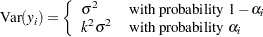where $\text{[math]}$ . The parameter $\text{[math]}$ is called the contamination coefficient. The value of $\text{[math]}$ is the prior probability of contamination for the $\text{[math]}$ th observation. Based on the prior probability of contamination for each observation, the call gives the posterior probability of contamination for each observation and the posterior probability that the entire sample is uncontaminated.

Box and Meyer (1986) suggest computing posterior probabilities of contamination for the analysis of saturated orthogonal factorial designs. Although these designs give uncorrelated estimates for effects, the significance of effects cannot be tested in an analysis of variance since there are no degrees of freedom for error. Box and Meyer suggest computing posterior probabilities of contamination for the effect estimates. The prior probabilities ( $\text{[math]}$ ) give the likelihood that an effect will be significant, and the contamination coefficient ( $\text{[math]}$ ) gives a measure of how large the significant effect will be. Box and Meyer recommend using $\text{[math]}$ and $\text{[math]}$ , implying that about 1 in 5 effects will be about 10 times larger than the remaining effects. To adequately explore posterior probabilities, examine them over a range of values for prior probabilities and a range of contamination coefficients.

If an independent estimate of $\text{[math]}$ is unavailable (as is the case when the $\text{[math]}$ s are effects from a saturated orthogonal design), use 0 for $\text{[math]}$ and $\text{[math]}$ in the BAYESACT call. Otherwise, the call assumes $\text{[math]}$ is proportional to the square root of a $\text{[math]}$ random variable with $\text{[math]}$ degrees of freedom. For example, if the $\text{[math]}$ s are estimated effects from an orthogonal design that is not saturated, then use the BAYESACT call with $\text{[math]}$ equal to the estimated standard error of the estimates and $\text{[math]}$ equal to the degrees of freedom for error.

From Bayes’ theorem, the posterior probability that $\text{[math]}$ is contaminated is

$\text{[math]}$

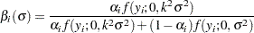for a given value of $\text{[math]}$ , where $\text{[math]}$ is the density of a normal distribution with mean $\text{[math]}$ and variance $\text{[math]}$ .

The probability that the sample is uncontaminated is

$\text{[math]}$

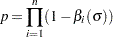Posterior probabilities that are independent of $\text{[math]}$ are derived by integrating $\text{[math]}$ and $\text{[math]}$ over a noninformative prior for $\text{[math]}$ . If an estimate of $\text{[math]}$ is available (when $\text{[math]}$ ), it is appropriately incorporated. Refer to Box and Meyer (1986) for details.

Examples

The statements

data;
   retain post1-post7 postnone;
   call bayesact(10,0,0,
          0.2,   0.2,   0.2,   0.2,   0.2,     0.2,   0.2,
      -5.4375,1.3875,8.2875,0.2625,1.7125,-11.4125,1.5875,
        post1, post2, post3, post4, post5,   post6, post7,
      postnone);
run;

return the following posterior probabilities:

POST1      0.42108
POST2      0.037412
POST3      0.53438
POST4      0.024679
POST5      0.050294
POST6      0.64329
POST7      0.044408
POSTNONE   0.28621

The probability that the sample is uncontaminated is 0.28621. A situation where this BAYESACT call would be appropriate is a saturated $\text{[math]}$ design in 8 runs, where the estimates for main effects are as shown in the function above (-5.4375, 1.3875, . . . , 1.5875).