The FREQ Procedure

The RISKDIFF option in the TABLES statement provides estimates of risks (binomial proportions) and risk differences for ![]() tables. This analysis might be appropriate when comparing the proportion of some characteristic for two groups, where row
1 and row 2 correspond to the two groups, and the columns correspond to two possible characteristics or outcomes. For example,
the row variable might be a treatment or dose, and the column variable might be the response. For more information, see Collett
(1991); Fleiss, Levin, and Paik (2003); Stokes, Davis, and Koch (2012).
tables. This analysis might be appropriate when comparing the proportion of some characteristic for two groups, where row
1 and row 2 correspond to the two groups, and the columns correspond to two possible characteristics or outcomes. For example,
the row variable might be a treatment or dose, and the column variable might be the response. For more information, see Collett
(1991); Fleiss, Levin, and Paik (2003); Stokes, Davis, and Koch (2012).
Let the frequencies of the ![]() table be represented as follows.
table be represented as follows.
|
Column 1 |
Column 2 |
Total |
|
|
Row 1 |
|
|
|
|
Row 2 |
|
|
|
|
Total |
|
|
n |
By default when you specify the RISKDIFF option, PROC FREQ provides estimates of the row 1 risk (proportion), the row 2 risk,
the overall risk, and the risk difference for column 1 and for column 2 of the ![]() table. The risk difference is defined as the row 1 risk minus the row 2 risk. The risks are binomial proportions of their
rows (row 1, row 2, or overall), and the computation of their standard errors and Wald confidence limits follow the binomial
proportion computations, which are described in the section Binomial Proportion.
table. The risk difference is defined as the row 1 risk minus the row 2 risk. The risks are binomial proportions of their
rows (row 1, row 2, or overall), and the computation of their standard errors and Wald confidence limits follow the binomial
proportion computations, which are described in the section Binomial Proportion.
The column 1 risk for row 1 is the proportion of row 1 observations classified in column 1,
which estimates the conditional probability of the column 1 response, given the first level of the row variable. The column 1 risk for row 2 is the proportion of row 2 observations classified in column 1,
The overall column 1 risk is the proportion of all observations classified in column 1,
The column 1 risk difference compares the risks for the two rows, and it is computed as the column 1 risk for row 1 minus the column 1 risk for row 2,
The standard error of the column 1 risk for row i is computed as
The standard error of the overall column 1 risk is computed as
Where the two rows represent independent binomial samples, the standard error of the column 1 risk difference is computed as
The computations are similar for the column 2 risks and risk difference.
By default, the RISKDIFF option provides Wald asymptotic confidence limits for the risks (row 1, row 2, and overall) and the risk difference. By default, the RISKDIFF option also provides exact (Clopper-Pearson) confidence limits for the risks. You can suppress the display of this information by specifying the NORISKS riskdiff-option. You can specify riskdiff-options to request tests and other types of confidence limits for the risk difference. See the sections Risk Difference Confidence Limits and Risk Difference Tests for more information.
The risks are equivalent to the binomial proportions of their corresponding rows. This section describes the Wald confidence limits that are provided by default when you specify the RISKDIFF option. The BINOMIAL option provides additional confidence limit types and tests for risks (binomial proportions). See the sections Binomial Confidence Limits and Binomial Tests for details.
The Wald confidence limits are based on the normal approximation to the binomial distribution. PROC FREQ computes the Wald confidence limits for the risks and risk differences as
where Est is the estimate, ![]() is the
is the ![]() percentile of the standard normal distribution, and
percentile of the standard normal distribution, and ![]() is the standard error of the estimate. The confidence level
is the standard error of the estimate. The confidence level ![]() is determined by the value of the ALPHA= option; the default of ALPHA=0.05 produces 95% confidence limits.
is determined by the value of the ALPHA= option; the default of ALPHA=0.05 produces 95% confidence limits.
If you specify the CORRECT riskdiff-option, PROC FREQ includes continuity corrections in the Wald confidence limits for the risks and risk differences. The purpose of a continuity correction is to adjust for the difference between the normal approximation and the binomial distribution, which is discrete. See Fleiss, Levin, and Paik (2003) for more information. The continuity-corrected Wald confidence limits are computed as
where cc is the continuity correction. For the row 1 risk, ![]() ; for the row 2 risk,
; for the row 2 risk, ![]() ; for the overall risk,
; for the overall risk, ![]() ; and for the risk difference,
; and for the risk difference, ![]() . The column 1 and column 2 risks use the same continuity corrections.
. The column 1 and column 2 risks use the same continuity corrections.
By default when you specify the RISKDIFF option, PROC FREQ also provides exact (Clopper-Pearson) confidence limits for the column 1, column 2, and overall risks. These confidence limits are constructed by inverting the equal-tailed test that is based on the binomial distribution. See the section Exact (Clopper-Pearson) Confidence Limits for details.
You can request additional confidence limits for the risk difference by specifying the CL= riskdiff-option. Available confidence limit types include Agresti-Caffo, exact unconditional, Hauck-Anderson, Miettinen-Nurminen (score), Newcombe (hybrid-score), and Wald confidence limits. Continuity-corrected Newcombe and Wald confidence limits are also available.
The confidence coefficient for the confidence limits produced by the CL= riskdiff-option is ![]() %, where the value of
%, where the value of ![]() is determined by the ALPHA= option. The default of ALPHA=0.05 produces 95% confidence limits. This differs from the test-based
confidence limits that are provided with the equivalence, noninferiority, and superiority tests, which have a confidence coefficient
of
is determined by the ALPHA= option. The default of ALPHA=0.05 produces 95% confidence limits. This differs from the test-based
confidence limits that are provided with the equivalence, noninferiority, and superiority tests, which have a confidence coefficient
of ![]() % (Schuirmann, 1999). See the section Risk Difference Tests for details.
% (Schuirmann, 1999). See the section Risk Difference Tests for details.
The section Exact Unconditional Confidence Limits for the Risk Difference describes the computation of the exact confidence limits. The confidence limits are constructed by inverting two separate one-sided exact tests (tail method). By default, the tests are based on the unstandardized risk difference. If you specify the RISKDIFF(METHOD=SCORE) option, the tests are based on the score statistic.
The following sections describe the computation of the Agresti-Coull, Hauck-Anderson, Miettinen-Nurminen (score), Newcombe (hybrid-score), and Wald confidence limits for the risk difference.
Agresti-Caffo Confidence Limits The Agresti-Caffo confidence limits for the risk difference are computed as
where ![]() ,
, ![]() ,
,
and ![]() is the
is the ![]() percentile of the standard normal distribution.
percentile of the standard normal distribution.
The Agresti-Caffo interval adjusts the Wald interval for the risk difference by adding a pseudo-observation of each type (success and failure) to each sample. See Agresti and Caffo (2000) and Agresti and Coull (1998) for more information.
Hauck-Anderson Confidence Limits The Hauck-Anderson confidence limits for the risk difference are computed as
where ![]() and
and ![]() is the
is the ![]() percentile of the standard normal distribution. The standard error is computed from the sample proportions as
percentile of the standard normal distribution. The standard error is computed from the sample proportions as
The Hauck-Anderson continuity correction cc is computed as
See Hauck and Anderson (1986) for more information. The subsection “Hauck-Anderson Test” in the section Noninferiority Tests describes the corresponding noninferiority test.
Miettinen-Nurminen (Score) Confidence Limits
The Miettinen-Nurminen (score) confidence limits for the risk difference (Miettinen and Nurminen, 1985) are computed by inverting score tests for the risk difference. A score-based test statistic for the null hypothesis that
the risk difference equals ![]() can be expressed as
can be expressed as
where ![]() is the observed value of the risk difference (
is the observed value of the risk difference (![]() ),
),
and ![]() and
and ![]() are the maximum likelihood estimates of the row 1 and row 2 risks (proportions) under the restriction that the risk difference
is
are the maximum likelihood estimates of the row 1 and row 2 risks (proportions) under the restriction that the risk difference
is ![]() . For more information, see Miettinen and Nurminen (1985, pp. 215–216) and Miettinen (1985, chapter 12).
. For more information, see Miettinen and Nurminen (1985, pp. 215–216) and Miettinen (1985, chapter 12).
The ![]() % confidence interval for the risk difference consists of all values of
% confidence interval for the risk difference consists of all values of ![]() for which the score test statistic
for which the score test statistic ![]() falls in the acceptance region,
falls in the acceptance region,
where ![]() is the
is the ![]() percentile of the standard normal distribution. PROC FREQ finds the confidence limits by iterative computation, which stops
when the iteration increment falls below the convergence criterion or when the maximum number of iterations is reached, whichever
occurs first. By default, the convergence criterion is 0.00000001 and the maximum number of iterations is 100.
percentile of the standard normal distribution. PROC FREQ finds the confidence limits by iterative computation, which stops
when the iteration increment falls below the convergence criterion or when the maximum number of iterations is reached, whichever
occurs first. By default, the convergence criterion is 0.00000001 and the maximum number of iterations is 100.
By default, the Miettinen-Nurminen confidence limits include the bias correction factor ![]() in the computation of
in the computation of ![]() (Miettinen and Nurminen, 1985, p. 216). For more information, see Newcombe and Nurminen (2011). If you specify the CL=MN(CORRECT=NO) riskdiff-option, PROC FREQ does not include the bias correction factor in this computation (Mee, 1984). See also Agresti (2002, p. 77). The uncorrected confidence limits are labeled as “Miettinen-Nurminen-Mee” confidence limits in the displayed output.
(Miettinen and Nurminen, 1985, p. 216). For more information, see Newcombe and Nurminen (2011). If you specify the CL=MN(CORRECT=NO) riskdiff-option, PROC FREQ does not include the bias correction factor in this computation (Mee, 1984). See also Agresti (2002, p. 77). The uncorrected confidence limits are labeled as “Miettinen-Nurminen-Mee” confidence limits in the displayed output.
The maximum likelihood estimates of ![]() and
and ![]() , subject to the constraint that the risk difference is
, subject to the constraint that the risk difference is ![]() , are computed as
, are computed as
where
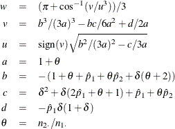
For more information, see Farrington and Manning (1990, p. 1453).
Newcombe Confidence Limits Newcombe (hybrid-score) confidence limits for the risk difference are constructed from the Wilson score confidence limits for each of the two individual proportions. The confidence limits for the individual proportions are used in the standard error terms of the Wald confidence limits for the proportion difference. See Newcombe (1998a) and Barker et al. (2001) for more information.
Wilson score confidence limits for ![]() and
and ![]() are the roots of
are the roots of
for ![]() . The confidence limits are computed as
. The confidence limits are computed as
See the section Wilson (Score) Confidence Limits for details.
Denote the lower and upper Wilson score confidence limits for ![]() as
as ![]() and
and ![]() , and denote the lower and upper confidence limits for
, and denote the lower and upper confidence limits for ![]() as
as ![]() and
and ![]() . The Newcombe confidence limits for the proportion difference (
. The Newcombe confidence limits for the proportion difference (![]() ) are computed as
) are computed as
![\begin{eqnarray*} d_ L = (\hat{p}_1 - \hat{p}_2) ~ - ~ \sqrt { ( \hat{p}_1 - L_1 )^2 ~ +~ ( U_2 - \hat{p}_2 )^2 } \\[0.10in] d_ U = (\hat{p}_1 - \hat{p}_2) ~ + ~ \sqrt { ( U_1 - \hat{p}_1 )^2 ~ +~ ( \hat{p}_2 - L_2 )^2 } \end{eqnarray*}](images/procstat_freq0309.png)
If you specify the CORRECT riskdiff-option, PROC FREQ provides continuity-corrected Newcombe confidence limits. By including a continuity correction of ![]() , the Wilson score confidence limits for the individual proportions are computed as the roots of
, the Wilson score confidence limits for the individual proportions are computed as the roots of
The continuity-corrected confidence limits for the individual proportions are then used to compute the proportion difference
confidence limits ![]() and
and ![]() .
.
Wald Confidence Limits The Wald confidence limits for the risk difference are computed as
where ![]() ,
, ![]() is the
is the ![]() percentile of the standard normal distribution. and the standard error is computed from the sample proportions as
percentile of the standard normal distribution. and the standard error is computed from the sample proportions as
If you specify the CORRECT riskdiff-option, the Wald confidence limits include a continuity correction cc,
where ![]() .
.
The subsection “Wald Test” in the section Noninferiority Tests describes the corresponding noninferiority test.
You can specify riskdiff-options to request tests of the risk (proportion) difference. You can request tests of equality, noninferiority, superiority, and equivalence for the risk difference. The test of equality is a standard Wald asymptotic test, available with or without a continuity correction. For noninferiority, superiority, and equivalence tests of the risk difference, the following test methods are provided: Wald (with and without continuity correction), Hauck-Anderson, Farrington-Manning (score), and Newcombe (with and without continuity correction). You can specify the test method with the METHOD= riskdiff-option. By default, PROC FREQ uses METHOD=WALD.
If you specify the EQUAL riskdiff-option, PROC FREQ computes a test of equality, or a test of the null hypothesis that the risk difference equals zero. For the column
1 (or 2) risk difference, this test can be expressed as ![]() versus the alternative
versus the alternative ![]() , where
, where ![]() denotes the column 1 (or 2) risk difference. PROC FREQ provides a Wald asymptotic test of equality. The test statistic is
computed as
denotes the column 1 (or 2) risk difference. PROC FREQ provides a Wald asymptotic test of equality. The test statistic is
computed as
By default, the standard error is computed from the sample proportions as
If you specify the VAR=NULL riskdiff-option, the standard error is based on the null hypothesis that the row 1 and row 2 risks are equal,
where ![]() estimates the overall column 1 risk.
estimates the overall column 1 risk.
If you specify the CORRECT riskdiff-option, PROC FREQ includes a continuity correction in the test statistic. If ![]() , the continuity correction is subtracted from
, the continuity correction is subtracted from ![]() in the numerator of the test statistic; otherwise, the continuity correction is added to the numerator. The value of the
continuity correction is
in the numerator of the test statistic; otherwise, the continuity correction is added to the numerator. The value of the
continuity correction is ![]() .
.
PROC FREQ computes one-sided and two-sided p-values for this test. When the test statistic z is greater than 0, PROC FREQ displays the right-sided p-value, which is the probability of a larger value occurring under the null hypothesis. The one-sided p-value can be expressed as
where Z has a standard normal distribution. The two-sided p-value is computed as ![]() .
.
If you specify the NONINF riskdiff-option, PROC FREQ provides a noninferiority test for the risk difference, or the difference between two proportions. The null hypothesis for the noninferiority test is
versus the alternative
where ![]() is the noninferiority margin. Rejection of the null hypothesis indicates that the row 1 risk is not inferior to the row 2
risk. See Chow, Shao, and Wang (2003) for more information.
is the noninferiority margin. Rejection of the null hypothesis indicates that the row 1 risk is not inferior to the row 2
risk. See Chow, Shao, and Wang (2003) for more information.
You can specify the value of ![]() with the MARGIN= riskdiff-option. By default,
with the MARGIN= riskdiff-option. By default, ![]() . You can specify the test method with the METHOD= riskdiff-option. The following methods are available for the risk difference noninferiority analysis: Wald (with and without continuity correction),
Hauck-Anderson, Farrington-Manning (score), and Newcombe (with and without continuity correction). The Wald, Hauck-Anderson,
and Farrington-Manning methods provide tests and corresponding test-based confidence limits; the Newcombe method provides
only confidence limits. If you do not specify METHOD=, PROC FREQ uses the Wald test by default.
. You can specify the test method with the METHOD= riskdiff-option. The following methods are available for the risk difference noninferiority analysis: Wald (with and without continuity correction),
Hauck-Anderson, Farrington-Manning (score), and Newcombe (with and without continuity correction). The Wald, Hauck-Anderson,
and Farrington-Manning methods provide tests and corresponding test-based confidence limits; the Newcombe method provides
only confidence limits. If you do not specify METHOD=, PROC FREQ uses the Wald test by default.
The confidence coefficient for the test-based confidence limits is ![]() % (Schuirmann, 1999). By default, if you do not specify the ALPHA= option, these are 90% confidence limits. You can compare the confidence limits
to the noninferiority limit, –
% (Schuirmann, 1999). By default, if you do not specify the ALPHA= option, these are 90% confidence limits. You can compare the confidence limits
to the noninferiority limit, –![]() .
.
The following sections describe the noninferiority analysis methods for the risk difference.
Wald Test If you specify the METHOD=WALD riskdiff-option, PROC FREQ provides an asymptotic Wald test of noninferiority for the risk difference. This is also the default method. The Wald test statistic is computed as
where (![]() ) estimates the risk difference and
) estimates the risk difference and ![]() is the noninferiority margin.
is the noninferiority margin.
By default, the standard error for the Wald test is computed from the sample proportions as
If you specify the VAR=NULL riskdiff-option, the standard error is based on the null hypothesis that the risk difference equals –![]() (Dunnett and Gent, 1977). The standard error is computed as
(Dunnett and Gent, 1977). The standard error is computed as
where
If you specify the CORRECT riskdiff-option, the test statistic includes a continuity correction. The continuity correction is subtracted from the numerator of the test
statistic if the numerator is greater than zero; otherwise, the continuity correction is added to the numerator. The value
of the continuity correction is ![]() .
.
The p-value for the Wald noninferiority test is ![]() , where Z has a standard normal distribution.
, where Z has a standard normal distribution.
Hauck-Anderson Test If you specify the METHOD=HA riskdiff-option, PROC FREQ provides the Hauck-Anderson test for noninferiority. The Hauck-Anderson test statistic is computed as
where ![]() and the standard error is computed from the sample proportions as
and the standard error is computed from the sample proportions as
The Hauck-Anderson continuity correction cc is computed as
The p-value for the Hauck-Anderson noninferiority test is ![]() , where Z has a standard normal distribution. See Hauck and Anderson (1986) and Schuirmann (1999) for more information.
, where Z has a standard normal distribution. See Hauck and Anderson (1986) and Schuirmann (1999) for more information.
Farrington-Manning (Score) Test
If you specify the METHOD=FM riskdiff-option, PROC FREQ provides the Farrington-Manning (score) test of noninferiority for the risk difference. A score test statistic
for the null hypothesis that the risk difference equals –![]() can be expressed as
can be expressed as
where ![]() is the observed value of the risk difference (
is the observed value of the risk difference (![]() ),
),
and ![]() and
and ![]() are the maximum likelihood estimates of the row 1 and row 2 risks (proportions) under the restriction that the risk difference
is –
are the maximum likelihood estimates of the row 1 and row 2 risks (proportions) under the restriction that the risk difference
is –![]() . The p-value for the noninferiority test is
. The p-value for the noninferiority test is ![]() , where Z has a standard normal distribution. For more information, see Miettinen and Nurminen (1985); Miettinen (1985); Farrington and Manning (1990); Dann and Koch (2005).
, where Z has a standard normal distribution. For more information, see Miettinen and Nurminen (1985); Miettinen (1985); Farrington and Manning (1990); Dann and Koch (2005).
The maximum likelihood estimates of ![]() and
and ![]() , subject to the constraint that the risk difference is –
, subject to the constraint that the risk difference is –![]() , are computed as
, are computed as
where
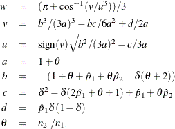
For more information, see Farrington and Manning (1990, p. 1453).
Newcombe Noninferiority Analysis
If you specify the METHOD=NEWCOMBE riskdiff-option, PROC FREQ provides a noninferiority analysis that is based on Newcombe hybrid-score confidence limits for the risk difference.
The confidence coefficient for the confidence limits is ![]() % (Schuirmann, 1999). By default, if you do not specify the ALPHA= option, these are 90% confidence limits. You can compare the confidence limits
with the noninferiority limit, –
% (Schuirmann, 1999). By default, if you do not specify the ALPHA= option, these are 90% confidence limits. You can compare the confidence limits
with the noninferiority limit, –![]() . If you specify the CORRECT riskdiff-option, the confidence limits includes a continuity correction. See the subsection “Newcombe Confidence Limits” in the section Risk Difference Confidence Limits for more information.
. If you specify the CORRECT riskdiff-option, the confidence limits includes a continuity correction. See the subsection “Newcombe Confidence Limits” in the section Risk Difference Confidence Limits for more information.
If you specify the SUP riskdiff-option, PROC FREQ provides a superiority test for the risk difference. The null hypothesis is
versus the alternative
where ![]() is the superiority margin. Rejection of the null hypothesis indicates that the row 1 proportion is superior to the row 2
proportion. You can specify the value of
is the superiority margin. Rejection of the null hypothesis indicates that the row 1 proportion is superior to the row 2
proportion. You can specify the value of ![]() with the MARGIN= riskdiff-option. By default,
with the MARGIN= riskdiff-option. By default, ![]() .
.
The superiority analysis is identical to the noninferiority analysis but uses a positive value of the margin ![]() in the null hypothesis. The superiority computations follow those in the section Noninferiority Tests by replacing –
in the null hypothesis. The superiority computations follow those in the section Noninferiority Tests by replacing –![]() by
by ![]() . See Chow, Shao, and Wang (2003) for more information.
. See Chow, Shao, and Wang (2003) for more information.
If you specify the EQUIV riskdiff-option, PROC FREQ provides an equivalence test for the risk difference, or the difference between two proportions. The null hypothesis for the equivalence test is
versus the alternative
where ![]() is the lower margin and
is the lower margin and ![]() is the upper margin. Rejection of the null hypothesis indicates that the two binomial proportions are equivalent. See Chow,
Shao, and Wang (2003) for more information.
is the upper margin. Rejection of the null hypothesis indicates that the two binomial proportions are equivalent. See Chow,
Shao, and Wang (2003) for more information.
You can specify the value of the margins ![]() and
and ![]() with the MARGIN= riskdiff-option. If you do not specify MARGIN=, PROC FREQ uses lower and upper margins of –0.2 and 0.2 by default. If you specify a single
margin value
with the MARGIN= riskdiff-option. If you do not specify MARGIN=, PROC FREQ uses lower and upper margins of –0.2 and 0.2 by default. If you specify a single
margin value ![]() , PROC FREQ uses lower and upper margins of –
, PROC FREQ uses lower and upper margins of –![]() and
and ![]() . You can specify the test method with the METHOD= riskdiff-option. The following methods are available for the risk difference equivalence analysis: Wald (with and without continuity correction),
Hauck-Anderson, Farrington-Manning (score), and Newcombe (with and without continuity correction). The Wald, Hauck-Anderson,
and Farrington-Manning methods provide tests and corresponding test-based confidence limits; the Newcombe method provides
only confidence limits. If you do not specify METHOD=, PROC FREQ uses the Wald test by default.
. You can specify the test method with the METHOD= riskdiff-option. The following methods are available for the risk difference equivalence analysis: Wald (with and without continuity correction),
Hauck-Anderson, Farrington-Manning (score), and Newcombe (with and without continuity correction). The Wald, Hauck-Anderson,
and Farrington-Manning methods provide tests and corresponding test-based confidence limits; the Newcombe method provides
only confidence limits. If you do not specify METHOD=, PROC FREQ uses the Wald test by default.
PROC FREQ computes two one-sided tests (TOST) for equivalence analysis
(Schuirmann, 1987). The TOST approach includes a right-sided test for the lower margin ![]() and a left-sided test for the upper margin
and a left-sided test for the upper margin ![]() . The overall p-value is taken to be the larger of the two p-values from the lower and upper tests.
. The overall p-value is taken to be the larger of the two p-values from the lower and upper tests.
The section Noninferiority Tests gives details about the Wald, Hauck-Anderson, Farrington-Manning (score), and Newcombe methods for the risk difference. The
lower margin equivalence test statistic takes the same form as the noninferiority test statistic but uses the lower margin
value ![]() in place of –
in place of –![]() . The upper margin equivalence test statistic take the same form as the noninferiority test statistic but uses the upper margin
value
. The upper margin equivalence test statistic take the same form as the noninferiority test statistic but uses the upper margin
value ![]() in place of –
in place of –![]() .
.
The test-based confidence limits for the risk difference are computed according to the equivalence test method that you select.
If you specify METHOD=WALD with VAR=NULL, or METHOD=FM, separate standard errors are computed for the lower and upper margin
tests. In this case, the test-based confidence limits are computed by using the maximum of these two standard errors. These
confidence limits have a confidence coefficient of ![]() % (Schuirmann, 1999). By default, if you do not specify the ALPHA= option, these are 90% confidence limits. You can compare the test-based confidence
limits to the equivalence limits,
% (Schuirmann, 1999). By default, if you do not specify the ALPHA= option, these are 90% confidence limits. You can compare the test-based confidence
limits to the equivalence limits, ![]() .
.
If you specify the RISKDIFF option in the EXACT statement, PROC FREQ provides exact unconditional confidence limits for the
risk difference. PROC FREQ computes the confidence limits by inverting two separate one-sided tests (tail method), where the
size of each test is at most ![]() and the confidence coefficient is at least
and the confidence coefficient is at least ![]() ). Exact conditional methods, described in the section Exact Statistics, do not apply to the risk difference due to the presence of a nuisance parameter (Agresti, 1992). The unconditional approach eliminates the nuisance parameter by maximizing the p-value over all possible values of the parameter (Santner and Snell, 1980).
). Exact conditional methods, described in the section Exact Statistics, do not apply to the risk difference due to the presence of a nuisance parameter (Agresti, 1992). The unconditional approach eliminates the nuisance parameter by maximizing the p-value over all possible values of the parameter (Santner and Snell, 1980).
By default, PROC FREQ uses the unstandardized risk difference as the test statistic in the confidence limit computations. If you specify the RISKDIFF(METHOD=SCORE) option, the procedure uses the score statistic (Chan and Zhang, 1999). The score statistic is a less discrete statistic than the raw risk difference and produces less conservative confidence limits (Agresti and Min, 2001). See also Santner et al. (2007) for comparisons of methods for computing exact confidence limits for the risk difference.
PROC FREQ computes the confidence limits as follows. The risk difference is defined as the difference between the row 1 and
row 2 risks (proportions), ![]() , and
, and ![]() and
and ![]() denote the row totals of the
denote the row totals of the ![]() table. The joint probability function for the table can be expressed in terms of the table cell frequencies, the risk difference,
and the nuisance parameter
table. The joint probability function for the table can be expressed in terms of the table cell frequencies, the risk difference,
and the nuisance parameter ![]() as
as
The ![]() % confidence limits for the risk difference are computed as
% confidence limits for the risk difference are computed as
where
![\begin{eqnarray*} P_ U(d_\ast ) & = & \sup _{p_2} ~ \bigl ( \sum _{A, T(a) \geq t_0} f( n_{11}, n_{21}; n_1, n_2, d_\ast , p_2 ) ~ \bigr ) \\[0.10in] P_ L(d_\ast ) & = & \sup _{p_2} ~ \bigl ( \sum _{A, T(a) \leq t_0} f( n_{11}, n_{21}; n_1, n_2, d_\ast , p_2 ) ~ \bigr ) \end{eqnarray*}](images/procstat_freq0345.png)
The set A includes all ![]() tables with row sums equal to
tables with row sums equal to ![]() and
and ![]() , and
, and ![]() denotes the value of the test statistic for table a in A. To compute
denotes the value of the test statistic for table a in A. To compute ![]() , the sum includes probabilities of those tables for which (
, the sum includes probabilities of those tables for which (![]() ), where
), where ![]() is the value of the test statistic for the observed table. For a fixed value of
is the value of the test statistic for the observed table. For a fixed value of ![]() ,
, ![]() is taken to be the maximum sum over all possible values of
is taken to be the maximum sum over all possible values of ![]() .
.
By default, PROC FREQ uses the unstandardized risk difference as the test statistic T. If you specify the RISKDIFF(METHOD=SCORE) option, the procedure uses the risk difference score statistic as the test statistic (Chan and Zhang, 1999). For information about the computation of the score statistic, see the section Risk Difference Confidence Limits. For more information, see Miettinen and Nurminen (1985) and Farrington and Manning (1990).
The BARNARD option in the EXACT statement provides an unconditional exact test for the risk (proportion) difference for ![]() tables. The reference set for the unconditional exact test consists of all
tables. The reference set for the unconditional exact test consists of all ![]() tables that have the same row sums as the observed table (Barnard, 1945, 1947, 1949). This differs from the reference set for exact conditional inference, which is restricted to the set of tables that have
the same row sums and the same column sums as the observed table. See the sections Fisher’s Exact Test and Exact Statistics for more information.
tables that have the same row sums as the observed table (Barnard, 1945, 1947, 1949). This differs from the reference set for exact conditional inference, which is restricted to the set of tables that have
the same row sums and the same column sums as the observed table. See the sections Fisher’s Exact Test and Exact Statistics for more information.
The test statistic is the standardized risk difference, which is computed as
where the risk difference d is defined as the difference between the row 1 and row 2 risks (proportions), ![]() ;
; ![]() and
and ![]() are the row 1 and row 2 totals, respectively; and
are the row 1 and row 2 totals, respectively; and ![]() is the overall proportion in column 1,
is the overall proportion in column 1, ![]() .
.
Under the null hypothesis that the risk difference is 0, the joint probability function for a table can be expressed in terms
of the table cell frequencies, the row totals, and the unknown parameter ![]() as
as
where ![]() is the common value of the risk (proportion).
is the common value of the risk (proportion).
PROC FREQ sums the table probabilities over the reference set for those tables where the test statistic is greater than or equal to the observed value of the test statistic. This sum can be expressed as
where the set A contains all ![]() tables with row sums equal to
tables with row sums equal to ![]() and
and ![]() , and
, and ![]() denotes the value of the test statistic for table a in A. The sum includes probabilities of those tables for which (
denotes the value of the test statistic for table a in A. The sum includes probabilities of those tables for which (![]() ), where
), where ![]() is the value of the test statistic for the observed table.
is the value of the test statistic for the observed table.
The sum Prob(![]() ) depends on the unknown value of
) depends on the unknown value of ![]() . To compute the exact p-value, PROC FREQ eliminates the nuisance parameter
. To compute the exact p-value, PROC FREQ eliminates the nuisance parameter ![]() by taking the maximum value of Prob(
by taking the maximum value of Prob(![]() ) over all possible values of
) over all possible values of ![]() ,
,
See Suissa and Shuster (1985) and Mehta and Senchaudhuri (2003).