| Introduction to Optimization |
| PROC OPTMODEL |
Modeling a Linear Programming Problem
Consider the candy manufacturer’s problem described in the section PROC OPTLP. You can formulate the problem using PROC OPTMODEL and solve it using the primal simplex solver as follows:
proc optmodel;

   /* declare variables */
   var choco, toffee;

   /* maximize objective function (profit) */
   maximize profit = 0.25*choco + 0.75*toffee;

   /* subject to constraints */
   con process1: 15*choco + 40*toffee    <= 27000;
   con process2:            56.25*toffee <= 27000;
   con process3: 18.75*choco             <= 27000;
   con process4: 12*choco + 50*toffee    <= 27000;
   /* solve LP using primal simplex solver */
   solve with lp / solver = primal_spx;
   /* display solution */
   print choco toffee;
quit;
The optimal objective value and the optimal solution are displayed in the following summary output:
| Solution Summary | |
|---|---|
| Solver | Primal Simplex |
| Objective Function | profit |
| Solution Status | Optimal |
| Objective Value | 475 |
| Iterations | 3 |
| Primal Infeasibility | 0 |
| Dual Infeasibility | 0 |
| Bound Infeasibility | 0 |
You can observe from the preceding example that PROC OPTMODEL provides an easy and intuitive way of modeling and solving mathematical programming models.
Modeling a Nonlinear Programming Problem
The following optimization problem illustrates how you can use some features of PROC OPTMODEL to formulate and solve nonlinear programming problems. The objective of the problem is to find coefficients for an approximation function that matches the values of a given function,  , at a set of points
  . The approximation is a rational function with degree
  in the numerator and denominator:
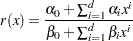 |
The problem can be formulated by minimizing the sum of squared errors at each point in :
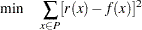 |
The following code implements this model. The function  is approximated over a set of points in the range 0 to 1. The function values are saved in a data set that is used by PROC OPTMODEL to set model parameters:
data points;
   /* generate data points */
   keep f x;
   do i = 0 to 100;
      x = i/100;
      f = 2**x;
      output;
   end;

proc optmodel;
   /* declare, read, and save our data points */
   set points;
   number f{points};
   read data points into points = [x] f;

   /* declare variables and model parameters */
   number d=1; /* linear polynomial */
   var a{0..d};
   var b{0..d} init 1;
   constraint fixb0: b[0] = 1;

   /* minimize sum of squared errors */
   min z=sum{x in points}
               ((a[0] + sum{i in 1..d} a[i]*x**i) /
                (b[0] + sum{i in 1..d} b[i]*x**i) - f[x])**2;

   /* solve and show coefficients */
   solve;
   print a b;
   quit;
The expression for the objective z is defined using operators that parallel the mathematical form. In this case the polynomials in the rational function are linear, so is equal to 1.
The constraint fixb0 forces the constant term of the rational function denominator, b[0], to equal 1. This causes the resulting coefficients to be normalized. The OPTMODEL presolver preprocesses the problem to remove the constraint. An unconstrained solver is used after substituting for b[0].
The SOLVE statement selects a solver, calls it, and displays the status. The PRINT command then prints the values of coefficient arrays a and b:
| Solution Summary | |
|---|---|
| Solver | NLPU/LBFGS |
| Objective Function | z |
| Solution Status | Optimal |
| Objective Value | 0.0000590999 |
| Iterations | 11 |
| Optimality Error | 6.5769853E-7 |
The approximation for between 0 and 1 is therefore
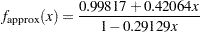 |
Copyright © SAS Institute, Inc. All Rights Reserved.