Interior Point Algorithmic Details

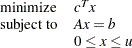
After preprocessing, the linear program to be solved is

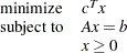This is the primal problem. The matrices , , and of NPSC have been renamed , , and , respectively, as these symbols are by convention used more, the problem to be solved is different from the original because of preprocessing, and there has been a change of primal variable to transform the LP into one whose variables have zero lower bounds. To simplify the algebra here, assume that variables have infinite upper bounds, and constraints are equalities. (Interior point algorithms do efficiently handle finite upper bounds, and it is easy to introduce primal slack variables to change inequalities into equalities.) The problem has variables; is a variable number; is an iteration number, and if used as a subscript or superscript it denotes "of iteration ".

There exists an equivalent problem, the dual problem, stated as

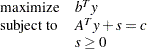where are dual variables, and are dual constraint slacks.

The interior point algorithm solves the system of equations to satisfy the Karush-Kuhn-Tucker (KKT) conditions for optimality:

where

(that is, if otherwise)

These are the conditions for feasibility, with the complementarity condition added. Complementarity forces the optimal objectives of the primal and dual to be equal, , as

Before the optimum is reached, a solution may not satisfy the KKT conditions:

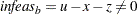
• Primal constraints may be violated, .

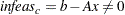• Dual constraints may be violated, .

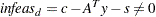• Complementarity may not be satisfied, . This is called the duality gap.

The interior point algorithm works by using Newton’s method to find a direction to move from the current solution toward a better solution:

where is the step length and is assigned a value as large as possible but not so large that an or is "too close" to zero. The direction in which to move is found using

To greatly improve performance, the third equation is changed to

where , the average complementarity, and

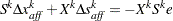
The effect now is to find a direction in which to move to reduce infeasibilities and to reduce the complementarity toward zero, but if any is too close to zero, it is "nudged out" to , and any that is larger than is "nudged into" . A close to or equal to 0.0 biases a direction toward the optimum, and a value of close to or equal to 1.0 "centers" the direction toward a point where all pairwise products . Such points make up the central path in the interior. Although centering directions make little, if any, progress in reducing and moving the solution closer to the optimum, substantial progress toward the optimum can usually be made in the next iteration.

The central path is crucial to why the interior point algorithm is so efficient. As is decreased, this path "guides" the algorithm to the optimum through the interior of feasible space. Without centering, the algorithm would find a series of solutions near each other close to the boundary of feasible space. Step lengths along the direction would be small and many more iterations would probably be required to reach the optimum.

That in a nutshell is the primal-dual interior point algorithm. Varieties of the algorithm differ in the way and are chosen and the direction adjusted during each iteration. A wealth of information can be found in the texts by Roos, Terlaky, and Vial (1997), Wright (1996), and Ye (1996).

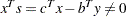
The calculation of the direction is the most time-consuming step of the interior point algorithm. Assume the th iteration is being performed, so the subscript and superscript can be dropped from the algebra:

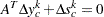
Rearranging the second equation,

Rearranging the third equation,

where

Equating these two expressions for and rearranging,

where

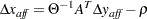
Substituting into the first direction equation,

, , , , and are calculated in that order. The hardest term is the factorization of the matrix to determine . Fortunately, although the values of are different for each iteration, the locations of the nonzeros in this matrix remain fixed; the nonzero locations are the same as those in the matrix . This is because is a diagonal matrix that has the effect of merely scaling the columns of .

The fact that the nonzeros in have a constant pattern is exploited by all interior point algorithms and is a major reason for their excellent performance. Before iterations begin, is examined and its rows and columns are symmetrically permuted so that during Cholesky factorization, the number of fill-ins created is smaller. A list of arithmetic operations to perform the factorization is saved in concise computer data structures (working with memory locations rather than actual numerical values). This is called symbolic factorization. During iterations, when memory has been initialized with numerical values, the operations list is performed sequentially. Determining how the factorization should be performed again and again is unnecessary.

The Primal-Dual Predictor-Corrector Interior Point Algorithm

The variant of the interior point algorithm implemented in PROC INTPOINT is a Primal-Dual Predictor-Corrector interior point algorithm. At first, Newton’s method is used to find a direction 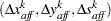to move, but calculated as if is zero, that is, as a step with no centering, known as an affine step:

where is the step length as before.

Complementarity is calculated at and compared with the complementarity at the starting point , and the success of the affine step is gauged. If the affine step was successful in reducing the complementarity by a substantial amount, the need for centering is not great, and in the following linear system is assigned a value close to zero. If, however, the affine step was unsuccessful, centering would be beneficial, and in the following linear system is assigned a value closer to 1.0. The value of is therefore adaptively altered depending on the progress made toward the optimum.

A second linear system is solved to determine a centering vector from :

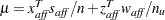
Then

where, as before, is the step length assigned a value as large as possible but not so large that an or is "too close" to zero.

Although the Predictor-Corrector variant entails solving two linear systems instead of one, fewer iterations are usually required to reach the optimum. The additional overhead of calculating the second linear system is small, as the factorization of the matrix has already been performed to solve the first linear system.

Interior Point: Upper Bounds

If the LP had upper bounds ( where is the upper bound vector), then the primal and dual problems, the duality gap, and the KKT conditions would have to be expanded.

The primal linear program to be solved is

where is split into and . Let be primal slack so that , and associate dual variables with these constraints. The interior point algorithm solves the system of equations to satisfy the Karush-Kuhn-Tucker (KKT) conditions for optimality:

These are the conditions for feasibility, with the complementarity conditions and added. Complementarity forces the optimal objectives of the primal and dual to be equal, 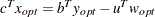, as

Before the optimum is reached, a solution might not satisfy the KKT conditions:

• Primal bound constraints may be violated, .

• Primal constraints may be violated, .

• Dual constraints may be violated, .

• Complementarity conditions may not be satisfied, or .

The calculations of the interior point algorithm can easily be derived in a fashion similar to calculations for when an LP has no upper bounds. See the paper by Lustig, Marsten, and Shanno (1992).

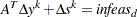
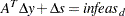
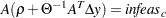
In some iteration , the affine step system that must be solved is

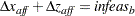
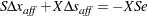
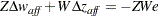
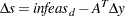
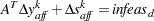
Therefore, the computations involved in solving the affine step are

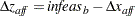
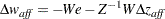
and is the step length as before.

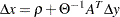
A second linear system is solved to determine a centering vector from :

where

, complementarity at the start of the iteration

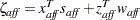, the affine complementarity

, the average complementarity

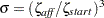
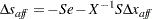
Therefore, the computations involved in solving the centering step are

Then

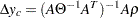
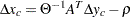
where, as before, is the step length assigned a value as large as possible but not so large that an , , , or is "too close" to zero.

The algebra in this section has been simplified by assuming that all variables have finite upper bounds. If the number of variables with finite upper bounds , you need to change the algebra to reflect that the and matrices have dimension or . Other computations need slight modification. For example, the average complementarity is

An important point is that any upper bounds can be handled by specializing the algorithm and not by generating the constraints and adding these to the main primal constraints .