The NETFLOW Procedure
Often all the details of a problem cannot be specified in a network model alone. In many of these cases, these details can be represented by the addition of side constraints to the model. Side constraints are a linear function of arc variables (variables containing flow through an arc) and nonarc variables (variables that are not part of the network). This enhancement to the basic network model allows for very general problems. In fact, any linear program can be represented with network models having these types of side constraints. The examples that follow help to clarify the notion of side constraints.
PROC NETFLOW enables you to specify side constraints. The data for a side constraint consist of coefficients of arcs and coefficients
of nonarc variables, a constraint type (that is, ![]() , =, or
, =, or ![]() ) and a right-hand-side value (rhs). A nonarc variable has a name, an objective function coefficient analogous to an arc cost,
an upper bound analogous to an arc capacity, and a lower bound analogous to an arc lower flow bound. PROC NETFLOW finds the
flow through the network and the values of any nonarc variables that minimize the total cost of the solution. Flow conservation
is met, flow through each arc is on or between the arc’s lower flow bound and capacity, the value of each nonarc variable
is on or between the nonarc’s lower and upper bounds, and the side constraints are satisfied. Note that, since many linear
programs have large embedded networks, PROC NETFLOW is an attractive alternative to the LP procedure in many cases.
) and a right-hand-side value (rhs). A nonarc variable has a name, an objective function coefficient analogous to an arc cost,
an upper bound analogous to an arc capacity, and a lower bound analogous to an arc lower flow bound. PROC NETFLOW finds the
flow through the network and the values of any nonarc variables that minimize the total cost of the solution. Flow conservation
is met, flow through each arc is on or between the arc’s lower flow bound and capacity, the value of each nonarc variable
is on or between the nonarc’s lower and upper bounds, and the side constraints are satisfied. Note that, since many linear
programs have large embedded networks, PROC NETFLOW is an attractive alternative to the LP procedure in many cases.
In order for arcs to be specified in side constraints, they must be named. By default, PROC NETFLOW names arcs using the names of the nodes at the head and tail of the arc. An arc is named with its tail node name followed by an underscore and its head node name. For example, an arc from node from to node to is called from_to.
Side constraints in network models fall into several categories that have special structure. They are frequently used when the flow through an arc must be proportional to the flow through another arc. Such constraints are called proportionality constraints and are useful in models where production is subject to refining or modification into different materials. The amount of each output, or any waste, evaporation, or reduction can be specified as a proportion of input.
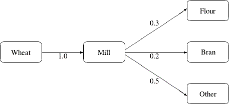
Typically the arcs near the supply nodes carry raw materials and the arcs near the demand nodes carry refined products. For example, in a model of the milling industry, the flow through some arcs may represent quantities of wheat. After the wheat is processed, the flow through other arcs might be flour. For others it might be bran. The side constraints model the relationship between the amount of flour or bran produced as a proportion of the amount of wheat milled. Some of the wheat can end up as neither flour, bran, nor any useful product, so this waste is drained away via arcs to a waste node.
Consider the network fragment in Figure 6.2. The arc Wheat_Mill conveys the wheat milled. The cost of flow on this arc is the milling cost. The capacity of this arc is the capacity of the
mill. The lower flow bound on this arc is the minimum quantity that must be milled for the mill to operate economically. The
constraints
![]()
Wheat_Mill ![]()
Mill_Flour ![]()
![]()
Wheat_Mill ![]()
Mill_Bran ![]()
force every unit of wheat that is milled to produce 0.3 units of flour and 0.2 units of bran. Note that it is not necessary to specify the constraint
![]()
Wheat_Mill ![]()
Mill_Other ![]()
since flow conservation implies that any flow that does not traverse through Mill_Flour or Mill_Bran must be conveyed through Mill_Other. And, computationally, it is better if this constraint is not specified, since there is one less side constraint and fewer
problems with numerical precision. Notice that the sum of the proportions must equal 1.0 exactly; otherwise, flow conservation
is violated.
Blending or quality constraints can also influence the recipes or proportions of ingredients that are mixed. For example, different raw materials can have different properties. In an application of the oil industry, the amount of products that are obtained could be different for each type of crude oil. Furthermore, fuel might have a minimum octane requirement or limited sulphur or lead content, so that a blending of crudes is needed to produce the product.
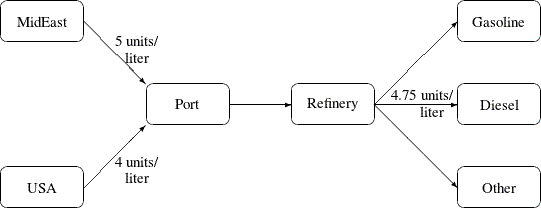
The network fragment in Figure 6.3 shows an example of this.
The arcs MidEast_Port and USA_Port convey crude oil from the two sources. The arc Port_Refinery represents refining while the arcs Refinery_Gasoline and Refinery_Diesel carry the gas and diesel produced. The proportionality constraints
![]()
Port_Refinery ![]()
Refinery_Gasoline ![]()
![]()
Port_Refinery ![]()
Refinery_Diesel ![]()
capture the restrictions for producing gasoline and diesel from crude. Suppose that, if only crude from the Middle East is used, the resulting diesel would contain 5 units of sulphur per liter. If only crude from the USA is used, the resulting diesel would contain 4 units of sulphur per liter. Diesel can have at most 4.75 units of sulphur per liter. Some crude from the USA must be used if Middle East crude is used in order to meet the 4.75 sulphur per liter limit. The side constraint to model this requirement is
![]()
MidEast_Port ![]()
USA_Port ![]()
Port_Refinery ![]()
![]()
Since Port_Refinery = MidEast_Port ![]()
USA_Port, flow conservation allows this constraint to be simplified to
![]()
MidEast_Port ![]()
USA_Port ![]() 0.0
0.0
If, for example, 120 units of crude from the Middle East is used, then at least 40 units of crude from the USA must be used. The preceding constraint is simplified because you assume that the sulphur concentration of diesel is proportional to the sulphur concentration of the crude mix. If this is not the case, the relation
![]()
Port_Refinery = Refinery_Diesel
is used to obtain
![]()
MidEast_Port ![]()
USA_Port ![]()
Refinery_Diesel![]()
![]()
which equals
![]()
MidEast_Port ![]()
USA_Port ![]()
Refinery_Diesel ![]() 0.0
0.0
An example similar to this Oil Industry problem is solved in the section Introductory Example.
Side constraints are also used in models in which there are capacities on transportation or some other shared resource, or there are limits on overall production or demand in multicommodity, multidivisional or multiperiod problems. Each commodity, division or period can have a separate network coupled to one main system by the side constraints. Side constraints are used to combine the outputs of subdivisions of a problem (either commodities, outputs in distinct time periods, or different process streams) to meet overall demands or to limit overall production or expenditures. This method is more desirable than doing separate local optimizations for individual commodity, process, or time networks and then trying to establish relationships between each when determining an overall policy if the global constraint is not satisfied. Of course, to make models more realistic, side constraints may be necessary in the local problems.
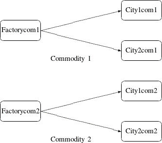
Figure 6.4 shows two network fragments. They represent identical production and distribution sites of two different commodities. Suffix
com1 represents commodity 1 and suffix com2 represents commodity 2. The nodes Factorycom1 and Factorycom2 model the same factory, and nodes City1com1 and City1com2 model the same location, city 1. Similarly, City2com1 and City2com2 are the same location, city 2. Suppose that commodity 1 occupies 2 cubic meters, commodity 2 occupies 3 cubic meters, the
truck dispatched to city 1 has a capacity of 200 cubic meters, and the truck dispatched to city 2 has a capacity of 250 cubic
meters. How much of each commodity can be loaded onto each truck? The side constraints for this case are
![]()
Factorycom1_City1com1 ![]()
Factorycom2_City1com2 ![]() 200
200
![]()
Factorycom1_City2com1 ![]()
Factorycom2_City2com2 ![]() 250
250
In many cases, the flow through an arc might actually represent the flow or movement of a commodity from place to place or from time period to time period. However, sometimes an arc is included in the network as a method of capturing some aspect of the problem that you would not normally think of as part of a network model. For example, in a multiprocess, multiproduct model (Figure 6.5), there might be subnetworks for each process and each product. The subnetworks can be joined together by a set of arcs that have flows that represent the amount of product j produced by process i. To model an upper limit constraint on the total amount of product j that can be produced, direct all arcs carrying product j to a single node and from there through a single arc. The capacity of this arc is the upper limit of product j production. It is preferable to model this structure in the network rather than to include it in the side constraints because the efficiency of the optimizer is affected less by a reasonable increase in the size of the network.
It is often a good strategy when starting a project to use a small network formulation and then use that model as a framework upon which to add detail. For example, in the multiprocess, multiproduct model, you might start with the network depicted in Figure 6.5. Then, for example, the process subnetwork can be enhanced to include the distribution of products. Other phases of the operation could be included by adding more subnetworks. Initially, these subnetworks can be single nodes, but in subsequent studies they can be expanded to include greater detail.
The NETFLOW procedure accepts the side constraints in the same dense and sparse formats that the LP procedure provides. Although PROC LP can solve network problems, the NETFLOW procedure generally solves network flow problems more efficiently than PROC LP.


