| Covariance Matrix |
The COV= option must be specified to compute an approximate covariance matrix for the parameter estimates under asymptotic theory for least squares, maximum-likelihood, or Bayesian estimation, with or without corrections for degrees of freedom as specified by the VARDEF= option.
Two groups of six different forms of covariance matrices (and therefore approximate standard errors) can be computed corresponding to the following two situations:
-
The LSQ statement is specified, which means that least squares estimates are being computed:

-
The MIN or MAX statement is specified, which means that maximum-likelihood or Bayesian estimates are being computed:
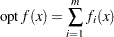
where
 is either
  or
or  .
.
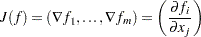
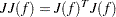
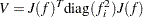
In either case, the following matrices are used:
 |
 |
 |
 |
 |
where
 |
For unconstrained minimization, or when none of the final parameter estimates are subjected to linear equality or active inequality constraints, the formulas of the six types of covariance matrices are as follows:
COV |
MIN or MAX Statement |
LSQ Statement |
|
1 |
M |
|
|
2 |
H |
|
|
3 |
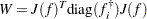
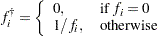
J |
|
|
4 |
B |
|
|
5 |
E |
|
|
6 |
U |
|
|
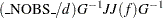

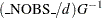


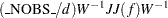

The value of  depends on the VARDEF= option and on the value of the _NOBS_ variable:
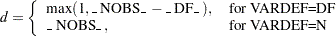 |
where _DF_ is either set in the program statements or set by default to  (the number of parameters) and _NOBS_ is either set in the program statements or set by default to nobs
  mfun, where nobs is the number of observations in the data set and mfun is the number of functions listed in the LSQ, MIN, or MAX statement.
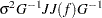
The value  depends on the specification of the SIGSQ= option and on the value of :
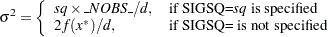 |
where  is the value of the objective function at the optimal parameter estimates
  .
.
The two groups of formulas distinguish between two situations:
For least squares estimates, the error variance can be estimated from the objective function value and is used in three of the six different forms of covariance matrices. If you have an independent estimate of the error variance, you can specify it with the SIGSQ= option.
For maximum-likelihood or Bayesian estimates, the objective function should be the logarithm of the likelihood or of the posterior density when using the MAX statement.
For minimization, the inversion of the matrices in these formulas is done so that negative eigenvalues are considered zero, resulting always in a positive semidefinite covariance matrix.
In small samples, estimates of the covariance matrix based on asymptotic theory are often too small and should be used with caution.
If the final parameter estimates are subjected to  linear equality or active linear inequality constraints, the formulas of the covariance matrices are modified similar to Gallant (1987) and Cramer (1986, p. 38) and additionally generalized for applications with singular matrices. In the constrained case, the value of used in the scalar factor is defined by
 |
where  is the number of active constraints and _NOBS_ is set as in the unconstrained case.
For minimization, the covariance matrix should be positive definite; for maximization it should be negative definite. There are several options available to check for a rank deficiency of the covariance matrix:
-
The ASINGULAR=, MSINGULAR=, and VSINGULAR= options can be used to set three singularity criteria for the inversion of the matrix
 needed to compute the covariance matrix, when is either the Hessian or one of the crossproduct Jacobian matrices. The singularity criterion used for the inversion is
where
 is the diagonal pivot of the matrix , and ASING, VSING and MSING are the specified values of the ASINGULAR=, VSINGULAR=, and MSINGULAR= options. The default values are
 ASING: the square root of the smallest positive double precision value
MSING:
 E
E if the SINGULAR= option is not specified and
  otherwise, where
  is the machine precision
 VSING:
E if the SINGULAR= option is not specified and the value of SINGULAR otherwise
Note: In many cases, a normalized matrix
 is decomposed and the singularity criteria are modified correspondingly.
 -
If the matrix
is found singular in the first step, a generalized inverse is computed. Depending on the G4= option, a generalized inverse is computed that satisfies either all four or only two Moore-Penrose conditions. If the number of parameters of the application is less than or equal to G4= , a G4 inverse is computed; otherwise only a G2 inverse is computed. The G4 inverse is computed by (the computationally very expensive but numerically stable) eigenvalue decomposition; the G2 inverse is computed by Gauss transformation. The G4 inverse is computed using the eigenvalue decomposition
  , where
  is the orthogonal matrix of eigenvectors and
  is the diagonal matrix of eigenvalues,
  . If the PEIGVAL option is specified, the eigenvalues
  are displayed. The G4 inverse of is set to
where the diagonal matrix
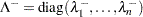 is defined using the COVSING= option:
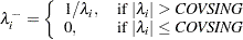
If the COVSING= option is not specified, the
 smallest eigenvalues are set to zero, where is the number of rank deficiencies found in the first step.
For optimization techniques that do not use second-order derivatives, the covariance matrix is usually computed using finite-difference approximations of the derivatives. By specifying TECH=NONE, any of the covariance matrices can be computed using analytical derivatives. The covariance matrix specified by the COV= option can be displayed (using the PCOV option) and is written to the OUTEST= data set.