Curve Fitting: Fitting a Curve to a Set of Data Points
PROC OPTMODEL Statements and Output
The following PROC OPTMODEL statements declare an index set and parameters and then read the input data:
proc optmodel;
   set POINTS;
   num x {POINTS};
   num y {POINTS};
   read data xy_data into POINTS=[_N_] x y;
The following NUM statement declares the order parameter, which is later set to 1 for Problems (1) and (2) and set to 2 for Problem (3):
   num order;
   var Beta {0..order};
   impvar Estimate {i in POINTS}
      = Beta[0] + sum {k in 1..order} Beta[k] * x[i]^k;
The following statements encode the linearization of the  norm:
norm:
   var Surplus {POINTS} >= 0;
   var Slack {POINTS} >= 0;
   min Objective1 = sum {i in POINTS} (Surplus[i] + Slack[i]);
   con Abs_dev_con {i in POINTS}:
      Estimate[i] - Surplus[i] + Slack[i] = y[i];
The following statements (which are not used but are shown here for comparison) encode an alternative linearization of the
norm that requires half as many variables but twice as many constraints:
   var AbsDeviation {POINTS} >= 0;
   min Objective1 = sum {i in POINTS} AbsDeviation[i];
   con Abs_dev_con1 {i in POINTS}:
      AbsDeviation[i] >= Estimate[i] - y[i];
   con Abs_dev_con2 {i in POINTS}:
      AbsDeviation[i] >= y[i] - Estimate[i];
The following additional declarations encode the linearization of the  norm:
norm:
   var MinMax;
   min Objective2 = MinMax;
   con MinMax_con {i in POINTS}:
      MinMax >= Surplus[i] + Slack[i];
The following statements (which are not used but match the formulation in Williams (1999)) encode an alternative linearization
of the norm that requires the same number of variables but twice as many constraints:
   var MinMax;
   min Objective2 = MinMax;
   con MinMax_con1 {i in POINTS}:
      MinMax >= Surplus[i];
   con MinMax_con2 {i in POINTS}:
      MinMax >= Slack[i];
The following NUM statements use the ABS function, the .sol variable suffix, and the MAX aggregation operator to compute the two norms from the optimal solution:
   num sum_abs_dev = sum {i in POINTS} abs(Estimate[i].sol - y[i]);
   num max_abs_dev = max {i in POINTS} abs(Estimate[i].sol - y[i]);
The following PROBLEM statement specifies the variables, objective, and constraints for minimization:
   problem L1 include
      Beta Surplus Slack
      Objective1
      Abs_dev_con;
The following PROBLEM statement specifies the additional variables, objective, and constraints for minimization:
   problem Linf from L1 include
      MinMax
      Objective2
      MinMax_con;
The following statements specify a straight line fit, switch the focus to problem L1, solve Problem (1), print the results, and store the y-values that are predicted by the optimal solution:
   order = 1;
   use problem L1;
   solve;
   print sum_abs_dev max_abs_dev;
   print Beta;
   print x y Estimate Surplus Slack;
   create data sol_data1 from [POINTS] x y Estimate;
Figure 11.1 shows the output from the linear programming solver for Problem (1).
Figure 11.1: Output from Linear Programming Solver for Problem (1)
| Problem Summary | |
|---|---|
| Objective Sense | Minimization |
| Objective Function | Objective1 |
| Objective Type | Linear |
| Number of Variables | 40 |
| Bounded Above | 0 |
| Bounded Below | 38 |
| Bounded Below and Above | 0 |
| Free | 2 |
| Fixed | 0 |
| Number of Constraints | 19 |
| Linear LE (<=) | 0 |
| Linear EQ (=) | 19 |
| Linear GE (>=) | 0 |
| Linear Range | 0 |
| Constraint Coefficients | 75 |
| [1] | x | y | Estimate | Surplus | Slack |
|---|---|---|---|---|---|
| 1 | 0.0 | 1.0 | 0.58125 | 0.00000 | 0.41875 |
| 2 | 0.5 | 0.9 | 0.90000 | 0.00000 | 0.00000 |
| 3 | 1.0 | 0.7 | 1.21875 | 0.51875 | 0.00000 |
| 4 | 1.5 | 1.5 | 1.53750 | 0.03750 | 0.00000 |
| 5 | 1.9 | 2.0 | 1.79250 | 0.00000 | 0.20750 |
| 6 | 2.5 | 2.4 | 2.17500 | 0.00000 | 0.22500 |
| 7 | 3.0 | 3.2 | 2.49375 | 0.00000 | 0.70625 |
| 8 | 3.5 | 2.0 | 2.81250 | 0.81250 | 0.00000 |
| 9 | 4.0 | 2.7 | 3.13125 | 0.43125 | 0.00000 |
| 10 | 4.5 | 3.5 | 3.45000 | 0.00000 | 0.05000 |
| 11 | 5.0 | 1.0 | 3.76875 | 2.76875 | 0.00000 |
| 12 | 5.5 | 4.0 | 4.08750 | 0.08750 | 0.00000 |
| 13 | 6.0 | 3.6 | 4.40625 | 0.80625 | 0.00000 |
| 14 | 6.6 | 2.7 | 4.78875 | 2.08875 | 0.00000 |
| 15 | 7.0 | 5.7 | 5.04375 | 0.00000 | 0.65625 |
| 16 | 7.6 | 4.6 | 5.42625 | 0.82625 | 0.00000 |
| 17 | 8.5 | 6.0 | 6.00000 | 0.00000 | 0.00000 |
| 18 | 9.0 | 6.8 | 6.31875 | 0.00000 | 0.48125 |
| 19 | 10.0 | 7.3 | 6.95625 | 0.00000 | 0.34375 |
The following statements switch the focus to problem Linf, solve Problem (2), print the results, and store the y-values that are predicted by the optimal solution:
   use problem Linf;
   solve;
   print sum_abs_dev max_abs_dev;
   print Beta;
   print x y Estimate Surplus Slack;
   create data sol_data2 from [POINTS] x y Estimate;
Figure 11.2 shows the output from the linear programming solver for Problem (2).
Figure 11.2: Output from Linear Programming Solver for Problem (2)
| Problem Summary | |
|---|---|
| Objective Sense | Minimization |
| Objective Function | Objective2 |
| Objective Type | Linear |
| Number of Variables | 41 |
| Bounded Above | 0 |
| Bounded Below | 38 |
| Bounded Below and Above | 0 |
| Free | 3 |
| Fixed | 0 |
| Number of Constraints | 38 |
| Linear LE (<=) | 0 |
| Linear EQ (=) | 19 |
| Linear GE (>=) | 19 |
| Linear Range | 0 |
| Constraint Coefficients | 132 |
| [1] | x | y | Estimate | Surplus | Slack |
|---|---|---|---|---|---|
| 1 | 0.0 | 1.0 | -0.4000 | 0.000 | 1.4000 |
| 2 | 0.5 | 0.9 | -0.0875 | 0.000 | 0.9875 |
| 3 | 1.0 | 0.7 | 0.2250 | 0.000 | 0.4750 |
| 4 | 1.5 | 1.5 | 0.5375 | 0.000 | 0.9625 |
| 5 | 1.9 | 2.0 | 0.7875 | 0.000 | 1.2125 |
| 6 | 2.5 | 2.4 | 1.1625 | 0.000 | 1.2375 |
| 7 | 3.0 | 3.2 | 1.4750 | 0.000 | 1.7250 |
| 8 | 3.5 | 2.0 | 1.7875 | 0.000 | 0.2125 |
| 9 | 4.0 | 2.7 | 2.1000 | 0.000 | 0.6000 |
| 10 | 4.5 | 3.5 | 2.4125 | 0.000 | 1.0875 |
| 11 | 5.0 | 1.0 | 2.7250 | 1.725 | 0.0000 |
| 12 | 5.5 | 4.0 | 3.0375 | 0.000 | 0.9625 |
| 13 | 6.0 | 3.6 | 3.3500 | 0.000 | 0.2500 |
| 14 | 6.6 | 2.7 | 3.7250 | 1.025 | 0.0000 |
| 15 | 7.0 | 5.7 | 3.9750 | 0.000 | 1.7250 |
| 16 | 7.6 | 4.6 | 4.3500 | 0.000 | 0.2500 |
| 17 | 8.5 | 6.0 | 4.9125 | 0.000 | 1.0875 |
| 18 | 9.0 | 6.8 | 5.2250 | 0.000 | 1.5750 |
| 19 | 10.0 | 7.3 | 5.8500 | 0.000 | 1.4500 |
The following statements specify a quadratic curve fit, solve both parts of Problem (3), print the results, and store the y-values that are predicted by the optimal solutions:
   order = 2;
   use problem L1;
   solve;
   print sum_abs_dev max_abs_dev;
   print Beta;
   print x y Estimate Surplus Slack;
   create data sol_data3 from [POINTS] x y Estimate;

   use problem Linf;
   solve;
   print sum_abs_dev max_abs_dev;
   print Beta;
   print x y Estimate Surplus Slack;
   create data sol_data4 from [POINTS] x y Estimate;
quit;
Figure 11.3 shows the output from the linear programming solver for the first part of Problem (3).
Figure 11.3: Output from Linear Programming Solver for First Part of Problem (3)
| Problem Summary | |
|---|---|
| Objective Sense | Minimization |
| Objective Function | Objective1 |
| Objective Type | Linear |
| Number of Variables | 41 |
| Bounded Above | 0 |
| Bounded Below | 38 |
| Bounded Below and Above | 0 |
| Free | 3 |
| Fixed | 0 |
| Number of Constraints | 19 |
| Linear LE (<=) | 0 |
| Linear EQ (=) | 19 |
| Linear GE (>=) | 0 |
| Linear Range | 0 |
| Constraint Coefficients | 93 |
| [1] | x | y | Estimate | Surplus | Slack |
|---|---|---|---|---|---|
| 1 | 0.0 | 1.0 | 0.98235 | 0.00000 | 0.017647 |
| 2 | 0.5 | 0.9 | 1.13804 | 0.23804 | 0.000000 |
| 3 | 1.0 | 0.7 | 1.31059 | 0.61059 | 0.000000 |
| 4 | 1.5 | 1.5 | 1.50000 | 0.00000 | 0.000000 |
| 5 | 1.9 | 2.0 | 1.66367 | 0.00000 | 0.336329 |
| 6 | 2.5 | 2.4 | 1.92941 | 0.00000 | 0.470588 |
| 7 | 3.0 | 3.2 | 2.16941 | 0.00000 | 1.030588 |
| 8 | 3.5 | 2.0 | 2.42627 | 0.42627 | 0.000000 |
| 9 | 4.0 | 2.7 | 2.70000 | 0.00000 | 0.000000 |
| 10 | 4.5 | 3.5 | 2.99059 | 0.00000 | 0.509412 |
| 11 | 5.0 | 1.0 | 3.29804 | 2.29804 | 0.000000 |
| 12 | 5.5 | 4.0 | 3.62235 | 0.00000 | 0.377647 |
| 13 | 6.0 | 3.6 | 3.96353 | 0.36353 | 0.000000 |
| 14 | 6.6 | 2.7 | 4.39520 | 1.69520 | 0.000000 |
| 15 | 7.0 | 5.7 | 4.69647 | 0.00000 | 1.003529 |
| 16 | 7.6 | 4.6 | 5.16861 | 0.56861 | 0.000000 |
| 17 | 8.5 | 6.0 | 5.92235 | 0.00000 | 0.077647 |
| 18 | 9.0 | 6.8 | 6.36471 | 0.00000 | 0.435294 |
| 19 | 10.0 | 7.3 | 7.30000 | 0.00000 | 0.000000 |
Figure 11.4 shows the output from the linear programming solver for the second part of Problem (3).
Figure 11.4: Output from Linear Programming Solver for Second Part of Problem (3)
| Problem Summary | |
|---|---|
| Objective Sense | Minimization |
| Objective Function | Objective2 |
| Objective Type | Linear |
| Number of Variables | 42 |
| Bounded Above | 0 |
| Bounded Below | 38 |
| Bounded Below and Above | 0 |
| Free | 4 |
| Fixed | 0 |
| Number of Constraints | 38 |
| Linear LE (<=) | 0 |
| Linear EQ (=) | 19 |
| Linear GE (>=) | 19 |
| Linear Range | 0 |
| Constraint Coefficients | 150 |
| [1] | x | y | Estimate | Surplus | Slack |
|---|---|---|---|---|---|
| 1 | 0.0 | 1.0 | 2.4750 | 1.47500 | 0.00000 |
| 2 | 0.5 | 0.9 | 2.1938 | 1.29375 | 0.00000 |
| 3 | 1.0 | 0.7 | 1.9750 | 1.27500 | 0.00000 |
| 4 | 1.5 | 1.5 | 1.8188 | 0.31875 | 0.00000 |
| 5 | 1.9 | 2.0 | 1.7388 | 0.00000 | 0.26125 |
| 6 | 2.5 | 2.4 | 1.6938 | 0.00000 | 0.70625 |
| 7 | 3.0 | 3.2 | 1.7250 | 0.00000 | 1.47500 |
| 8 | 3.5 | 2.0 | 1.8188 | 0.00000 | 0.18125 |
| 9 | 4.0 | 2.7 | 1.9750 | 0.00000 | 0.72500 |
| 10 | 4.5 | 3.5 | 2.1938 | 0.00000 | 1.30625 |
| 11 | 5.0 | 1.0 | 2.4750 | 1.47500 | 0.00000 |
| 12 | 5.5 | 4.0 | 2.8188 | 0.00000 | 1.18125 |
| 13 | 6.0 | 3.6 | 3.2250 | 0.00000 | 0.37500 |
| 14 | 6.6 | 2.7 | 3.7950 | 1.09500 | 0.00000 |
| 15 | 7.0 | 5.7 | 4.2250 | 0.00000 | 1.47500 |
| 16 | 7.6 | 4.6 | 4.9450 | 0.34500 | 0.00000 |
| 17 | 8.5 | 6.0 | 6.1938 | 0.19375 | 0.00000 |
| 18 | 9.0 | 6.8 | 6.9750 | 0.17500 | 0.00000 |
| 19 | 10.0 | 7.3 | 8.7250 | 1.42500 | 0.00000 |
You can find a higher-order polynomial fit simply by increasing the value of the order parameter. The dimensions of the Beta and Estimate variables are automatically updated when order changes.
The following PROC SGPLOT statements use the output data sets that are created by PROC OPTMODEL to display the results from Problems (1) and (2) in one plot:
data plot1;
   merge sol_data1(rename=(Estimate=Line1)) sol_data2(rename=(Estimate=Line2));
run;

proc sgplot data=plot1;
   scatter x=x y=y;
   series x=x y=Line1 / curvelabel;
   series x=x y=Line2 / curvelabel;
run;
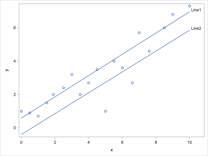
Figure 11.5 shows the regression lines for Problems (1) and (2), as on page 319 of Williams (1999).
Figure 11.5: Regression Lines for Problems (1) and (2)
The following PROC SGPLOT statements use the output data sets that are created by PROC OPTMODEL to display the results from both parts of Problem (3) in one plot:
data plot2;
   merge sol_data3(rename=(Estimate=Curve1))
      sol_data4(rename=(Estimate=Curve2));
run;

proc sgplot data=plot2;
   scatter x=x y=y;
   series x=x y=Curve1 / curvelabel;
   series x=x y=Curve2 / curvelabel;
run;
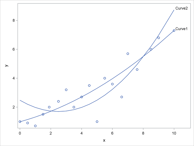
Figure 11.6 shows the regression curves for Problem (3), as on page 319 of Williams (1999).
Figure 11.6: Regression Curves for Problem (3)