Milk Collection: How to Route and Assign Milk Collection Lorries to Farms
The first several PROC OPTMODEL statements declare index sets and parameters and then read the input data:
proc optmodel;
   set NODES;
   num east {NODES};
   num north {NODES};
   num frequency {NODES};
   num requirement {NODES};
   read data farm_data into NODES=[_N_] east north frequency requirement;

   set EDGES = {i in NODES, j in NODES: i < j};
   num distance {<i,j> in EDGES} =
      &distance_scale * sqrt((east[i]-east[j])^2+(north[i]-north[j])^2);

   set DAYS = 1..&num_days;
The following model declaration statements correspond directly to the mathematical programming formulation that is described earlier:
   var UseNode {NODES, DAYS} binary;
   var UseEdge {EDGES, DAYS} binary;

   min TotalDistance
      = sum {<i,j> in EDGES, d in DAYS} distance[i,j] * UseEdge[i,j,d];

   con Capacity_con {d in DAYS}:
      sum {i in NODES} requirement[i] * UseNode[i,d] <= &capacity;

   con Frequency_con {i in NODES}:
      sum {d in DAYS} UseNode[i,d] = frequency[i];

   con Two_match {k in NODES, d in DAYS}:
      sum {<i,j> in EDGES: k in {i,j}} UseEdge[i,j,d] = 2 * UseNode[k,d];
The following statements declare optional symmetry-breaking constraints to reduce the number of essentially identical branch-and-bound nodes that are explored by the mixed integer linear programming solver:
   /* several alternatives for symmetry-breaking constraints */
*  con Symmetry {d in DAYS diff {1}}:
      sum {<i,j> in EDGES} distance[i,j] * UseEdge[i,j,d]
   <= sum {<i,j> in EDGES} distance[i,j] * UseEdge[i,j,d-1];
*  con Symmetry {d in DAYS diff {1}}:
      sum {i in NODES} requirement[i] * UseNode[i,d]
   <= sum {i in NODES} requirement[i] * UseNode[i,d-1];
   con Symmetry {d in DAYS diff {1}}:
      sum {i in NODES} UseNode[i,d]
   <= sum {i in NODES} UseNode[i,d-1];
Williams (1999) breaks symmetry instead by fixing ![]() . The symmetry-breaking constraints shown here apply to the general formulation with any number of days and arbitrary frequencies.
. The symmetry-breaking constraints shown here apply to the general formulation with any number of days and arbitrary frequencies.
In SAS/OR 13.1, the mixed integer linear programming solver automatically detects and exploits symmetry without you having to explicitly declare such symmetry-breaking constraints. You can control the aggressiveness of symmetry detection by using the SYMMETRY= option in the SOLVE WITH MILP statement.
The following statements declare the subtour elimination constraints:
   num num_subtours init 0;
   /* subset of nodes not containing depot node */
   set SUBTOUR {1..num_subtours};
   /* if node k in SUBTOUR[s] is used on day d, then
      must use at least two edges across partition induced by SUBTOUR[s] */
   con Subtour_elimination {s in 1..num_subtours, k in SUBTOUR[s], d in DAYS}:
      sum {i in NODES diff SUBTOUR[s], j in SUBTOUR[s]: <i,j> in EDGES}
         UseEdge[i,j,d]
    + sum {i in SUBTOUR[s], j in NODES diff SUBTOUR[s]: <i,j> in EDGES}
         UseEdge[i,j,d]
   >= 2 * UseNode[k,d];
The following statements declare the index sets and parameters that are needed to detect violated subtour elimination constraints:
   num iter init 0;
   num num_components {DAYS};
   set NODES_TEMP;
   set <num,num> EDGES_SOL {1..iter, DAYS};
   num component_id {NODES_TEMP};
   set COMPONENT_IDS;
   set COMPONENT {COMPONENT_IDS};
   num ci;
   num cj;
The following DO UNTIL loop implements dynamic generation of subtour elimination constraints (“row generation”):
   /* loop until each day's support graph is connected */
   do until (and {d in DAYS} num_components[d] = 1);
      iter = iter + 1;
      solve;
      /* find connected components for each day */
      for {d in DAYS} do;
         NODES_TEMP = {i in NODES: UseNode[i,d].sol > 0.5};
         EDGES_SOL[iter,d] = {<i,j> in EDGES: UseEdge[i,j,d].sol > 0.5};
         /* initialize each node to its own component */
         COMPONENT_IDS = NODES_TEMP;
         num_components[d] = card(NODES_TEMP);
         for {i in NODES_TEMP} do;
            component_id[i] = i;
            COMPONENT[i] = {i};
         end;
         /* if i and j are in different components, merge the two components */
         for {<i,j> in EDGES_SOL[iter,d]} do;
            ci = component_id[i];
            cj = component_id[j];
            if ci ne cj then do;
               /* update smaller component */
               if card(COMPONENT[ci]) < card(COMPONENT[cj]) then do;
                  for {k in COMPONENT[ci]} component_id[k] = cj;
                  COMPONENT[cj] = COMPONENT[cj] union COMPONENT[ci];
                  COMPONENT_IDS = COMPONENT_IDS diff {ci};
               end;
               else do;
                  for {k in COMPONENT[cj]} component_id[k] = ci;
                  COMPONENT[ci] = COMPONENT[ci] union COMPONENT[cj];
                  COMPONENT_IDS = COMPONENT_IDS diff {cj};
               end;
            end;
         end;
         num_components[d] = card(COMPONENT_IDS);
         put num_components[d]=;
         /* create subtour from each component not containing depot node */
         for {k in COMPONENT_IDS: &depot not in COMPONENT[k]} do;
            num_subtours = num_subtours + 1;
            SUBTOUR[num_subtours] = COMPONENT[k];
            put SUBTOUR[num_subtours]=;
         end;
      end;
      print capacity_con.body capacity_con.ub;
      print num_components;
   end;
The body of the loop calls the mixed integer linear programming solver, finds the connected components of the support graph of the resulting solution, and adds any subtours found. Note that the DO UNTIL loop contains no declaration statements. As the value of num_subtours changes, the SOLVE statement automatically updates the subtour elimination constraints. See Chapter 27 for an alternative approach that instead uses the SOLVE WITH NETWORK statement together with the CONCOMP option to find the connected components.
After the DO UNTIL loop terminates, the following statements output the edges that appear in each iteration of subtour elimination and write the value of iter to a SAS macro variable named num_iters:
   create data sol_data from
      [iter d i j]={it in 1..iter, d in DAYS, <i,j> in EDGES_SOL[it,d]}
      xi=east[i] yi=north[i] xj=east[j] yj=north[j];
   call symput('num_iters',put(iter,best.));
quit;
The following SAS macro calls PROC SGPLOT to plot the solution that results from each iteration:
%macro showPlots;
   %do iter = 1 %to &num_iters;
      %do d = 1 %to &num_days;
         /* create annotate data set to draw subtours */
         data sganno(keep=drawspace linethickness function x1 y1 x2 y2);
            retain drawspace "datavalue" linethickness 1;
            set sol_data(rename=(xi=x1 yi=y1 xj=x2 yj=y2));
            where iter = &iter and d = &d;
            function = 'line';
         run;

         title1 "iter = &iter, day = &d";
         title2;
         proc sgplot data=farm_data sganno=sganno;
            scatter y=north x=east / group=frequency datalabel=farm;
            xaxis display=(nolabel);
            yaxis display=(nolabel);
         run;
         quit;
      %end;
   %end;
%mend showPlots;
%showPlots;
Figure 23.2 and Figure 23.3 show the output from the mixed integer linear programming solver for the first iteration, before any subtour elimination constraints have been generated.
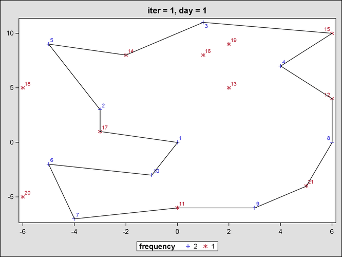
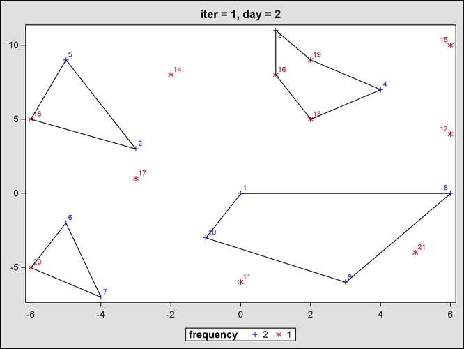
Figure 23.4 and Figure 23.5 show the output from the mixed integer linear programming solver for the second iteration, after the first round of subtour elimination constraints.
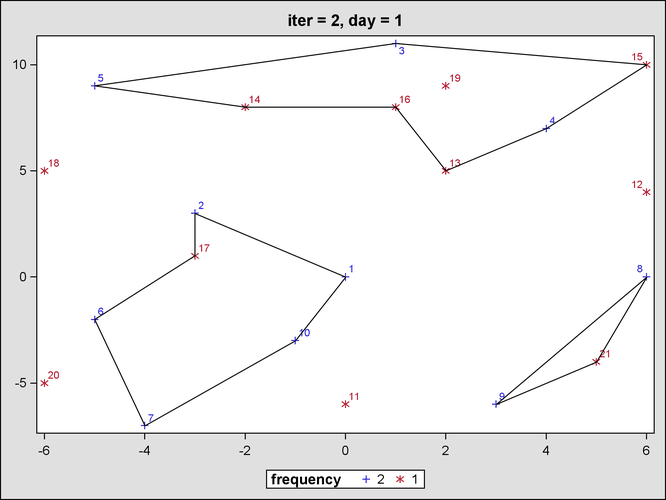
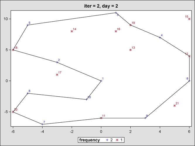
Figure 23.6 and Figure 23.7 show the output from the mixed integer linear programming solver for the third iteration, after the second round of subtour elimination constraints.
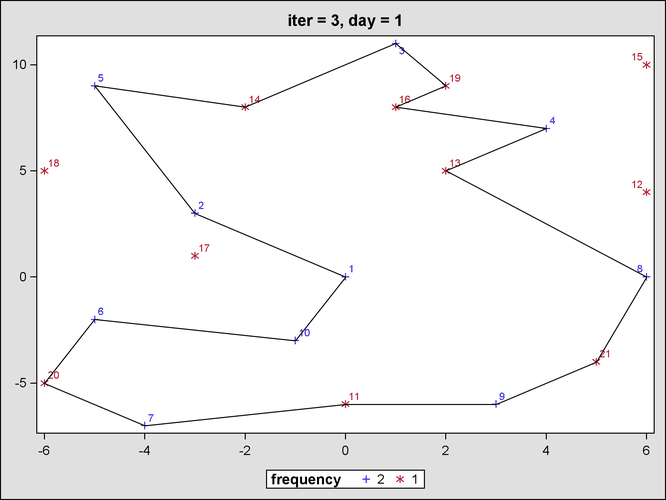
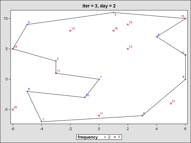
Since no more subtour elimination constraints are violated, the DO UNTIL loop terminates with an optimal solution. Figure 23.8 shows the final problem and solution summaries from the mixed integer linear programming solver.
Figure 23.8: Final Problem and Solution Summaries from Mixed Integer Linear Programming Solver
| Problem Summary | |
|---|---|
| Objective Sense | Minimization |
| Objective Function | TotalDistance |
| Objective Type | Linear |
| Number of Variables | 462 |
| Bounded Above | 0 |
| Bounded Below | 0 |
| Bounded Below and Above | 462 |
| Free | 0 |
| Fixed | 0 |
| Binary | 462 |
| Integer | 0 |
| Number of Constraints | 108 |
| Linear LE (<=) | 3 |
| Linear EQ (=) | 63 |
| Linear GE (>=) | 42 |
| Linear Range | 0 |
| Constraint Coefficients | 4192 |
| Solution Summary | |
|---|---|
| Solver | MILP |
| Algorithm | Branch and Cut |
| Objective Function | TotalDistance |
| Solution Status | Optimal |
| Objective Value | 1230.5623785 |
| Relative Gap | 0 |
| Absolute Gap | 0 |
| Primal Infeasibility | 8.881784E-16 |
| Bound Infeasibility | 6.661338E-16 |
| Integer Infeasibility | 6.661338E-16 |
| Best Bound | 1230.5623785 |
| Nodes | 1 |
| Iterations | 1449 |
| Presolve Time | 0.00 |
| Solution Time | 0.08 |
The optimal objective value differs slightly from the one given in Williams (1999), perhaps because of rounding of distances
by Williams.