The first several PROC OPTMODEL statements declare index sets and parameters and then read the input data:
proc optmodel;
   num n = &num_acids;
   set POSITIONS = 1..n;
   set HYDROPHOBIC;
   read data hydrophobic_data into HYDROPHOBIC=[position];
The following statement uses the MOD function to declare the set of hydrophobic pairs that can possibly be matched (because they are not contiguous and are an even number of positions apart):
   set PAIRS
      = {i in HYDROPHOBIC, j in HYDROPHOBIC: i + 1 < j and mod(j-i-1,2) = 0};
The following model declaration statements correspond directly to the mathematical programming formulation that is described earlier:
   /* IsFold[i] = 1 if fold occurs between positions i and i + 1; 0 otherwise */
   var IsFold {1..n-1} binary;

   /* IsMatch[i,j] = 1 if hydrophobic pair at positions i and j are matched;
      0 otherwise */
   var IsMatch {PAIRS} binary;

   /* maximize number of matches */
   max NumMatches = sum {<i,j> in PAIRS} IsMatch[i,j];

   /* if IsMatch[i,j] = 1 then IsFold[k] = 0 */
   con DoNotFold {<i,j> in PAIRS, k in i..j-1 diff {(i+j-1)/2}}:
      IsMatch[i,j] + IsFold[k] <= 1;

   /* if IsMatch[i,j] = 1 then IsFold[k] = 1 */
   con FoldHalfwayBetween {<i,j> in PAIRS}:
      IsMatch[i,j] <= IsFold[(i+j-1)/2];
The following statements call the mixed integer linear programming solver and print the positive variables in the resulting optimal solution:
   solve;
   print {i in 1..n-1: IsFold[i].sol > 0.5} IsFold;
   print {<i,j> in PAIRS: IsMatch[i,j].sol > 0.5} IsMatch;
Figure 28.4 shows the output from the mixed integer linear programming solver.
Figure 28.4: Output from Mixed Integer Linear Programming Solver
| Problem Summary | |
|---|---|
| Objective Sense | Maximization |
| Objective Function | NumMatches |
| Objective Type | Linear |
| Number of Variables | 124 |
| Bounded Above | 0 |
| Bounded Below | 0 |
| Bounded Below and Above | 124 |
| Free | 0 |
| Fixed | 0 |
| Binary | 124 |
| Integer | 0 |
| Number of Constraints | 1265 |
| Linear LE (<=) | 1265 |
| Linear EQ (=) | 0 |
| Linear GE (>=) | 0 |
| Linear Range | 0 |
| Constraint Coefficients | 2530 |
| Performance Information | |
|---|---|
| Execution Mode | Single-Machine |
| Number of Threads | 1 |
| Solution Summary | |
|---|---|
| Solver | MILP |
| Algorithm | Branch and Cut |
| Objective Function | NumMatches |
| Solution Status | Optimal |
| Objective Value | 10 |
| Relative Gap | 0 |
| Absolute Gap | 0 |
| Primal Infeasibility | 0 |
| Bound Infeasibility | 0 |
| Integer Infeasibility | 1E-6 |
| Best Bound | 10 |
| Nodes | 198 |
| Iterations | 4908 |
| Presolve Time | 0.05 |
| Solution Time | 1.28 |
| [1] | IsFold |
|---|---|
| 3 | 1 |
| 8 | 1 |
| 14 | 1 |
| 18 | 1 |
| 22 | 1 |
| 26 | 1 |
| 29 | 1 |
| 38 | 1 |
| [1] | [2] | IsMatch |
|---|---|---|
| 2 | 5 | 1 |
| 5 | 12 | 1 |
| 6 | 11 | 1 |
| 12 | 17 | 1 |
| 17 | 20 | 1 |
| 20 | 25 | 1 |
| 25 | 28 | 1 |
| 28 | 31 | 1 |
| 31 | 46 | 1 |
| 33 | 44 | 1 |
The optimal solution and objective value differ from Williams (2013), because of an error that will be corrected in a subsequent
printing by Wiley.
The following statements compute ![]() and
and ![]() coordinates for each position and write multiple output data sets to be used by the SGPLOT procedure:
coordinates for each position and write multiple output data sets to be used by the SGPLOT procedure:
   num x {POSITIONS};
   num y {POSITIONS};
   num xx init 0;
   num yy init 0;
   num dir init 1;
   for {i in POSITIONS} do;
      xx = xx + dir;
      x[i] = xx;
      y[i] = yy;
      if i = n or IsFold[i].sol > 0.5 then do;
         xx = xx + dir;
         dir = -dir;
         yy = yy - 1;
      end;
   end;
   create data plot_data from [i] x y is_hydrophobic=(i in HYDROPHOBIC);
   create data edge_data from [i]=(1..n-1)
      x1=x[i] y1=y[i] x2=x[i+1] y2=y[i+1] linepattern=1;
   create data match_data from [i j]={<i,j> in PAIRS: IsMatch[i,j].sol > 0.5}
      x1=x[i] y1=y[i] x2=x[j] y2=y[j] linepattern=2;
quit;
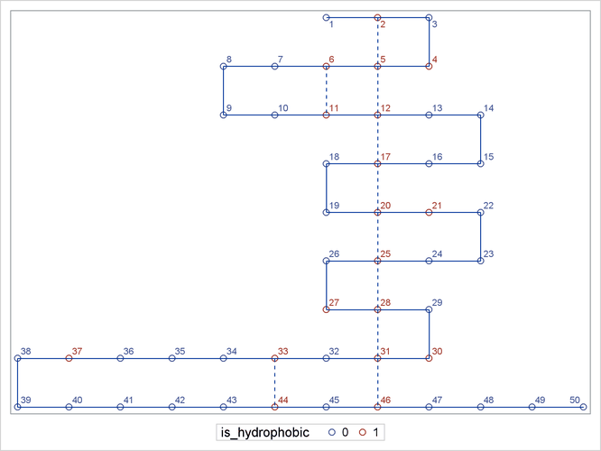
The following DATA step and PROC SGPLOT statements use the output data sets that are created by PROC OPTMODEL to display the optimal folding that corresponds to the MILP solution:
data sganno(drop=i j);
   retain drawspace "datavalue" linethickness 1;
   set edge_data match_data;
   function = 'line';
run;

proc sgplot data=plot_data sganno=sganno;
   scatter x=x y=y / group=is_hydrophobic datalabel=i;
   xaxis display=none;
   yaxis display=none;
run;
quit;
Figure 28.5 shows a plot of the optimal folding that corresponds to the MILP solution.