Example 3.11 10×10 Job Shop Scheduling Problem

This example is a job shop scheduling problem from Lawrence (1984). This test is also known as LA19 in the literature, and its optimal makespan is known to be 842 (Applegate and Cook; 1991). There are 10 jobs (J1–J10) and 10 machines (M0–M9). Every job must be processed on each of the 10 machines in a predefined sequence. The objective is to minimize the completion time of the last job to be processed, known as the makespan. The jobs are described in the data set raw by using the following statements.

/* jobs specification */
data raw (drop=i mid);
   do i=1 to 10;
      input mid _DURATION_ @;
      _RESOURCE_=compress('M'||put(mid,best.));
      output;
   end;
   datalines;
2  44  3   5  5  58  4  97  0   9  7  84  8  77  9  96  1  58  6  89
4  15  7  31  1  87  8  57  0  77  3  85  2  81  5  39  9  73  6  21
9  82  6  22  4  10  3  70  1  49  0  40  8  34  2  48  7  80  5  71
1  91  2  17  7  62  5  75  8  47  4  11  3   7  6  72  9  35  0  55
6  71  1  90  3  75  0  64  2  94  8  15  4  12  7  67  9  20  5  50
7  70  5  93  8  77  2  29  4  58  6  93  3  68  1  57  9   7  0  52
6  87  1  63  4  26  5   6  2  82  3  27  7  56  8  48  9  36  0  95
0  36  5  15  8  41  9  78  3  76  6  84  4  30  7  76  2  36  1   8
5  88  2  81  3  13  6  82  4  54  7  13  8  29  9  40  1  78  0  75
9  88  4  54  6  64  7  32  0  52  2   6  8  54  5  82  3   6  1  26
;

Each row in the DATALINES section specifies a job by 10 pairs of consecutive numbers. Each pair of numbers defines one task of the job, which represents the processing of a job on a machine. For each pair, the first number identifies the machine it executes on, and the second number is the duration. The order of the 10 pairs defines the sequence of the tasks for a job.

The following statements create the Activity data set actdata, which defines the activities, durations, and precedence constraints:

/* create the Activity data set */
data actdata (drop= i j);
   format _ACTIVITY_ $8. _SUCCESSOR_ $8.;
   set raw;
   _QTY_ = 1;
   i=mod(_n_-1,10)+1;
   j=int((_n_-1)/10)+1;
   _ACTIVITY_ = compress('J'||put(j,best.)||'P'||put(i,best.));
   JOB=j;
   TASK=i;
   if i LT 10 then
      _SUCCESSOR_ = compress('J'||put(j,best.)||'P'||put((i+1),best.));
   else
      _SUCCESSOR_ = ' ';
   output;   
run;

Had there been sufficient machine capacity, the jobs could have been processed according to a schedule as shown in Output 3.11.1. The minimum makespan would be 617—the time it takes to complete Job 1.

Output 3.11.1 Gantt Chart: Schedule for the Unconstrained Problem

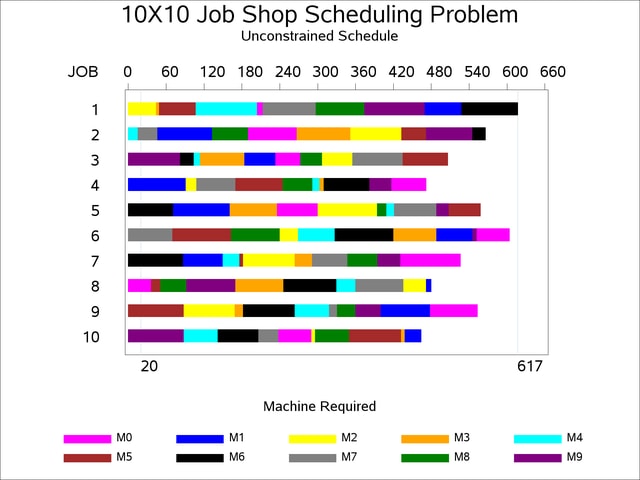
This schedule is infeasible when there is only a single instance of each machine. For example, at time period 20, the schedule requires two instances of each of the machines M6, M7, and M9.

In order to solve the resource-constrained schedule, the CLP procedure is invoked by using the following statements:

proc clp domain=[0,842]
         actdata=actdata
         schedout=sched_jobshop
         dpr=50
         restarts=150
         showprogress;
   schedule dur=842 edgefinder nf=1 nl=1;
run;

The edge-finder algorithm is activated with the EDGEFINDER option in the SCHEDULE statement. In addition, the edge-finding extensions for detecting whether a job cannot be the first or cannot be the last to be processed on a particular machine are invoked with the NF= and NL= options, respectively, in the SCHEDULE statement. The default activity selection and activity assignment strategies are used. A restart heuristic is used as the look-back method to handle recovery from failures. The DPR= option specifies that a total restart be performed after encountering 50 failures, and the RESTARTS= option limits the number of restarts to 150.

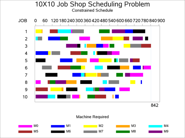
The resulting 842-time-period schedule is displayed in Output 3.11.2. Each row represents a job. Each segment represents a task (the processing of a job on a machine), which is also coded according to the executing machine. The mapping of the coding is indicated in the legend. Note that no machine is used by more than one job at any point in time.

Output 3.11.2 Gantt Chart: Optimal Resource-Constrained Schedule