Output Tables for the TEXTPARSE Statement :: SAS(R) LASR(TM) Analytic Server 2.4: Reference Guide

Sample Data and Program

The TEXTPARSE statement generates a summary table and up to seven temporary tables. The following program provides sample data and statements for getting started and then showing the basic layout for each of the temporary tables.

data getstart;
infile cards delimiter='|' missover;
length text $150;
input text$ docid$;

cards;
High-performance analytics hold the key to |d01
unlocking the unprecedented business value of big data.|d02
Organizations looking for optimal ways to gain insights|d03
from big data in shorter reporting windows are turning to SAS.|d04
As the gold-standard leader in business analytics |d05
for more than 36 years,|d06
SAS frees enterprises from the limitations of |d07
traditional computing and enables them |d08
to draw instant benefits from big data.|d09
Faster Time to Insight.|d10
From banking to retail to health care to insurance, |d11
SAS is helping industries glean insights from data |d12
that once took days or weeks in just hours, minutes, or seconds.|d13
It's all about getting to and analyzing relevant data faster.|d14
Revealing previously unseen patterns, sentiments, and relationships.|d15
Identifying unknown risks.|d16
And speeding the time to insights.|d17
High-Performance Analytics from SAS Combining industry-leading |d18
analytics software with high-performance computing technologies|d19
produces fast and precise answers to unsolvable problems|d20
and enables our customers to gain greater competitive advantage.|d21
SAS In-Memory Analytics eliminate the need for disk-based processing|d22
allowing for much faster analysis.|d23
SAS In-Database executes analytic logic into the database itself |d24
for improved agility and governance.|d25
SAS Grid Computing creates a centrally managed,|d26
shared environment for processing large jobs|d27
and supporting a growing number of users efficiently.|d28
Together, the components of this integrated, |d29
supercharged platform are changing the decision-making landscape|d30
and redefining how the world solves big data business problems.|d31
Big data is a popular term used to describe the exponential growth,|d32
availability and use of information,|d33
both structured and unstructured.|d34
Much has been written on the big data trend and how it can |d35
serve as the basis for innovation, differentiation and growth.|d36
run;

options set=TKTXTANIO_BINDAT_DIR="/opt/TKTGDat";

libname example sasiola host="grid001.example.com" port=10010 tag=hps;

data example.getstart;
  set getstart;
run;

proc imstat data=example.getstart;
  textparse var=text docid=docid entities=std reducef=2 
            select=(_all_) save=txtsummary;
run;

Computing singular value decomposition requires the input data to contain at least 25 documents and at least as many documents as there are machines in the cluster. By default, REDUCEF=4 but in this example is set to 2 to specify that a word only needs to appear twice to be kept for generating the term-by-document matrix. The default dimension for the singular-value decomposition is k=10 and the server generates ten topics.

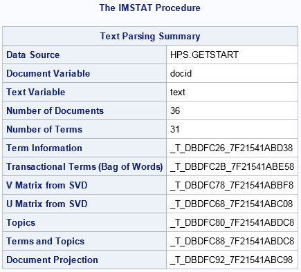
The TEXTPARSE statement produces the following output. The names of the temporary tables are reported and begin with _T_. These names (and the rest of the output in the table) is stored in a temporary buffer that is named TXTSUMMARY.

Because the IMSTAT procedure was used in interactive mode with a RUN statement instead of QUIT, the STORE statement can be used to create macro variables for the temporary table names as follows:

  store txtsummary( 6,2) as Terms;
  store txtsummary( 7,2) as Parent;
  store txtsummary( 8,2) as V;
  store txtsummary( 9,2) as U;
  store txtsummary(10,2) as Topics;
  store txtsummary(11,2) as TermsByTopics;
  store txtsummary(12,2) as DocPro;
run;

Each of the tables can then be accessed with a libref and the macro variable, such as example.&Terms.;. The following sections show how to access these tables.

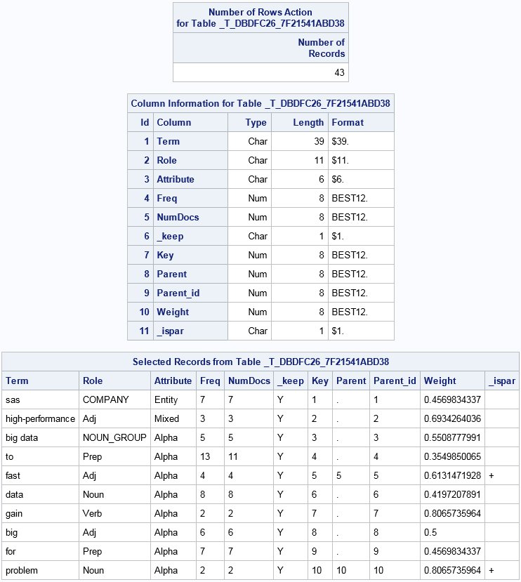
Terms Table

Based on the statements in the previous section, you can access the terms table as follows:

  table example.&Terms.;
  numrows;
  columninfo;
  where _ispar ne ".";
  fetch / format to=10;
run;

Note: Filtering out the observations where _Ispar is missing results in showing only the terms that are used in the subsequent singular-value decomposition and topic generation.

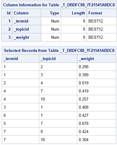
The following output shows the number of observations in the Terms table, the data structure, and details about the terms that are identified by the TEXTPARSE statement.

Number of observations, columns, and first 10 observations from the Terms table

Parent Table

The Parent table is also known as the bag of words or as the term document. It is a sparse representation of the term by document weights. It is the input to the singular-value decomposition (SVD). The SVD then reduces the dimensionality of the problem by focusing on the k dimensions with the largest singular values. It is essentially a dimension reduction technique.

  where; /* clear the _ispar filter that was in use */
  table example.&Parent.;
  numrows;
  columninfo;
  fetch / format to=10;
run;

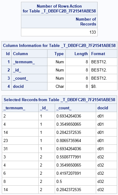
Number of observations, columns, and first 10 observations from the Parent table

There are 133 nonzero entries in the term × document matrix. The full matrix would be a 43 × 36 matrix.

There are four columns in the parent table. The _termnum_, and _id_ column are the term number and an internal identifier. Values in the _termnum_ column correspond to values in the Key column in the Terms table. The _count_ column represents the term weight. The last column is the document ID that corresponds to the DOCID= variable specified in the TEXTPARSE statement. In this example, it is named Docid.

SVD V Table

  table example.&V.;
  numrows;
  columninfo;
  fetch / format to=10;
run;

This table is one of the results of the singular-value decomposition of the sparse parent table (bag of words). The number of rows equals the number of documents in the input table. The number of columns equals the number of topics (the K= value of the SVD option) plus one for an ID variable.

Number of observations, columns, and first 10 observations from the V table

SVD U Table

  table example.&U.;
  numrows;
  columninfo;
  fetch / format to=10;
run;

This table contains the U matrix from the singular-value decomposition. The number of rows equals the number of terms in the SVD (31). The number of columns equals the number of topics (the K= value of the SVD option) plus an _ID_ column.

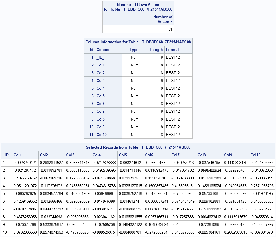
Number of observations, columns, and first 10 observations from the U table

Note: The U matrix produced by the TEXTPARSE statement in the server does not match the U matrix that is generated by the HPTMINE procedure for SAS Text Miner. The SAS LASR Analytic Server performs a varimax rotation on the matrix. This step is done by SAS Text Miner on the HPTMINE output with the FACTOR procedure.

Topics Table

  table example.&Topics;
  columninfo;
  fetch / format to=10;
run;

This table displays the topics identified by the server, the term weight cutoff for the topic, and a descriptive label formed from the terms in the topic with the highest weights. By default, five terms are used to label the topic. You can specify a different number with the NUMLABELS= option.

Column information and first 10 observations from the Topics table

Terms by Topic Table

  table example.&TermsByTopic;
  columninfo;
  fetch / format to=10;
run;

The terms-by-topic table is a sparse representation of the term-by-topic matrix.

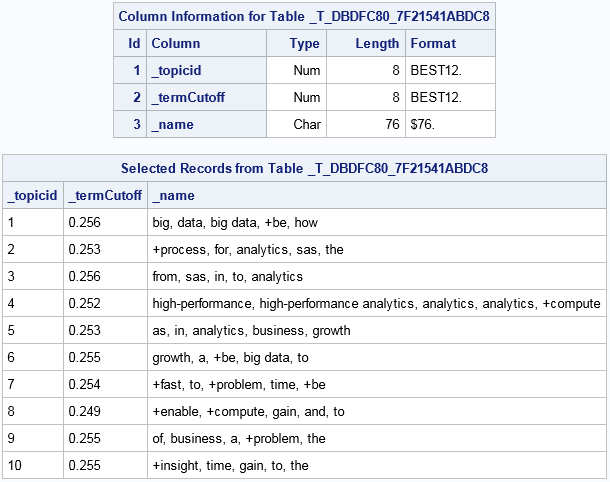
Column information and first 10 observations from the Terms by topic table

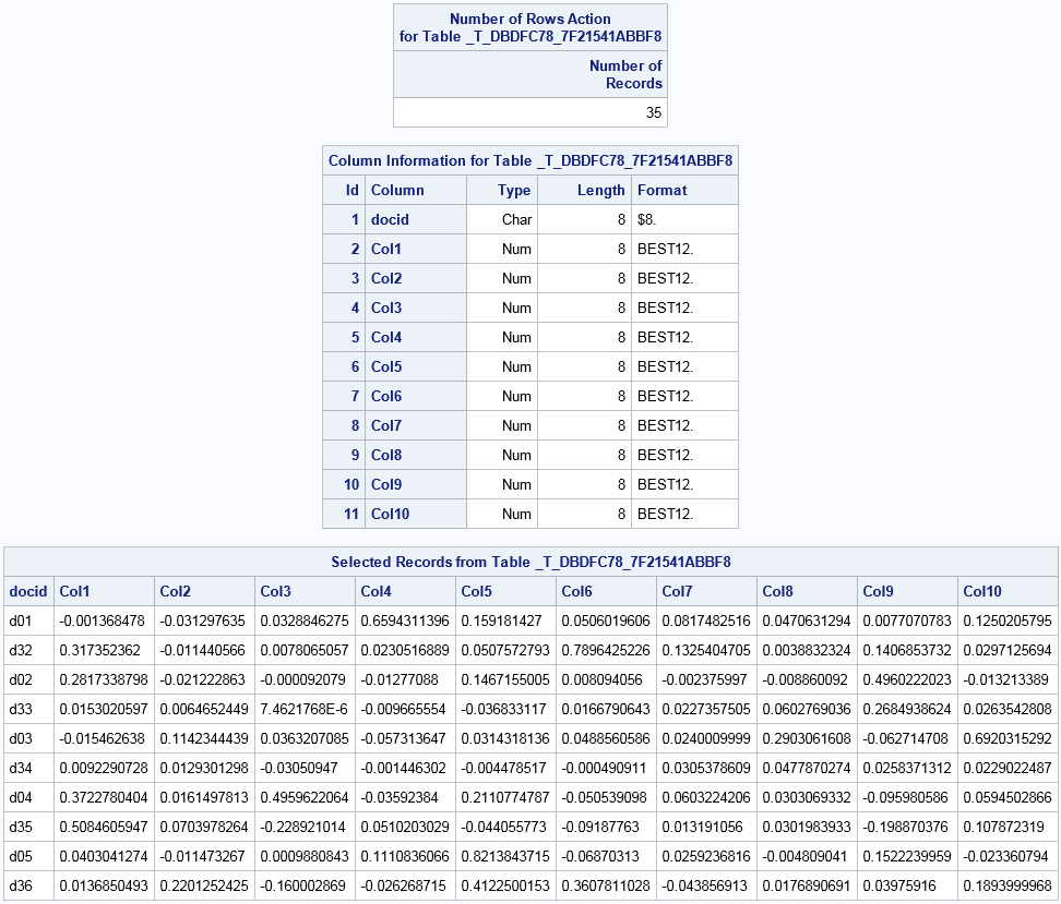
Document Projection Table

  table example.&DocPro.;
  columninfo;
  fetch / format to=10;
run;

The projected document contains at a minimum the document ID variable from the input table and the projection onto the topic space. The number of rows equals the number of documents in the input table. The number of columns equals the number of topics (the K= value of the SVD option) plus the document ID column. Each of the Col1 to Colk columns are the projections.

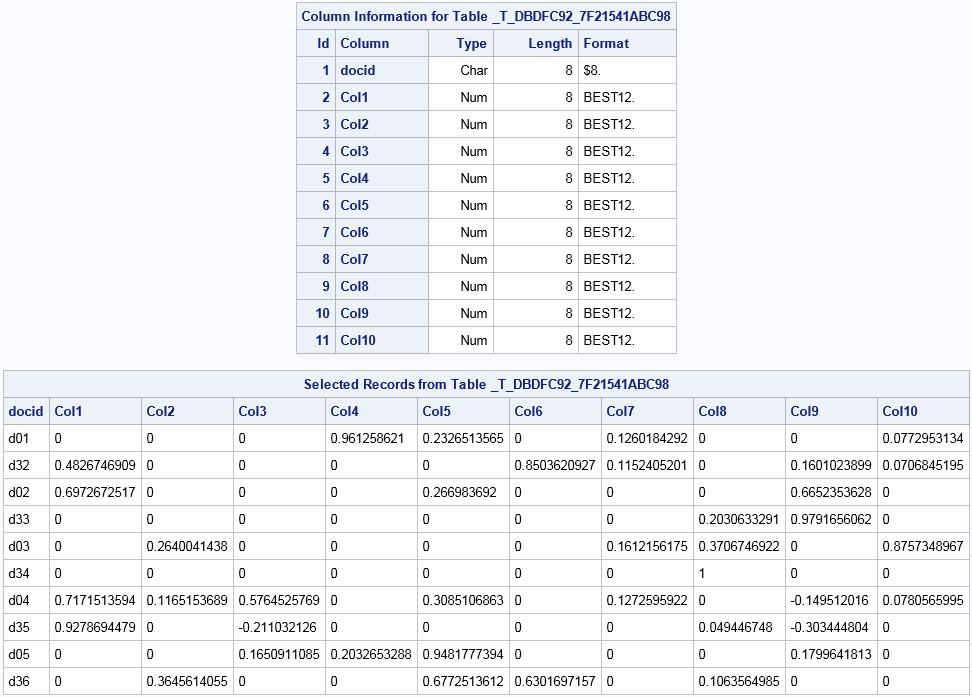
Column information and first 10 observations from the Document Projection table

You can request that other variables, beside the document ID variable, are transferred to the projected document table. If you do not transfer variables, then the document projection table is a candidate for a join with the input table on the document ID in order to associate the documents with their topic weights.