Robust Regression Examples
Example 13.5 Multivariate Location, Scale, and Outliers
This section analyzes the three regressors in the stack loss data of Brownlee (1965), which are defined in Example 13.2. As in the previous section, the LOAD MODULES=_ALL_ statement loads modules that are defined in the RobustMC.sas file.
%include sampsrc(robustmc);   /* define graphing modules */
proc iml;
load module=_all_;            /* load graphing modules */
By default, the MVE subroutine generates 2,000 randomly selected subsets in its search. The following call to the MVE subroutine uses all 5,985 subsets of four observations that can be chosen from the 21 observations:
   /* Obs X1  X2  X3   Y  Stack Loss data */
SL = { 1  80  27  89  42,
       2  80  27  88  37,
       3  75  25  90  37,
       4  62  24  87  28,
       5  62  22  87  18,
       6  62  23  87  18,
       7  62  24  93  19,
       8  62  24  93  20,
       9  58  23  87  15,
      10  58  18  80  14,
      11  58  18  89  14,
      12  58  17  88  13,
      13  58  18  82  11,
      14  58  19  93  12,
      15  50  18  89   8,
      16  50  18  86   7,
      17  50  19  72   8,
      18  50  19  79   8,
      19  50  20  80   9,
      20  56  20  82  15,
      21  70  20  91  15 };
x = SL[, 2:4]; y = SL[, 5];

optn = j(5,1,.);
optn[1] = 1;             /* print basic output */
optn[2] = 1;             /* print covariance matrices */
optn[5]= -1;             /* nrep: use all subsets */

ods select ClassicalMean ClassicalCov RobustMVELoc RobustMVEScatter;
call mve(sc, xmve, dist, optn, x);
ods select all;
Output 13.5.1 shows the classical and robust estimates of the location. Output 13.5.2 shows the classical and robust estimates of the scatter.
Output 13.5.1: Classical and Robust Estimates of the Location
Output 13.5.2: Classical and Robust Estimates of the Scatter
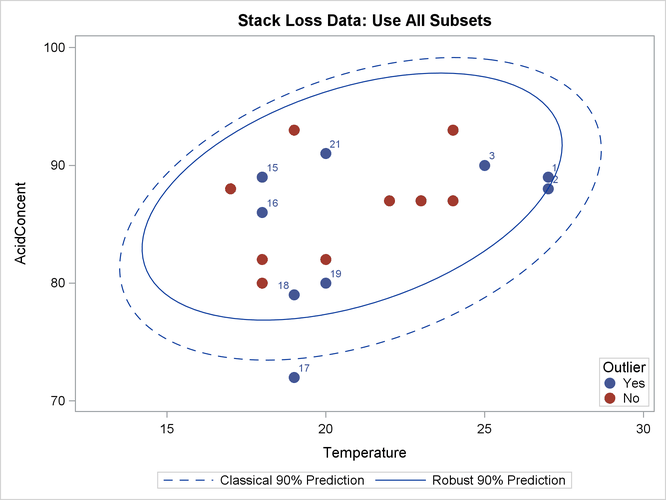
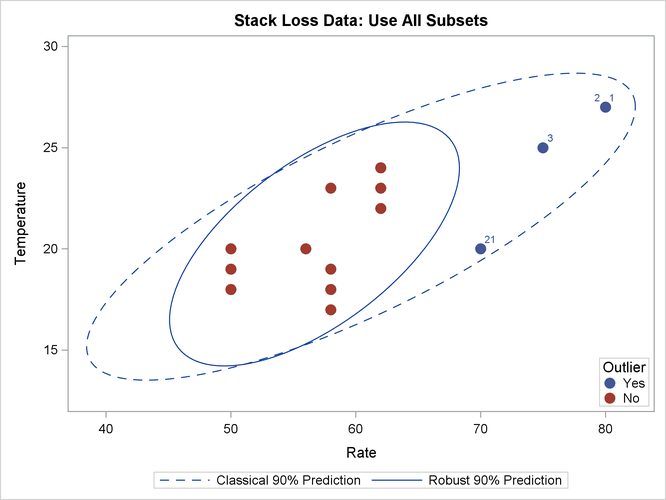
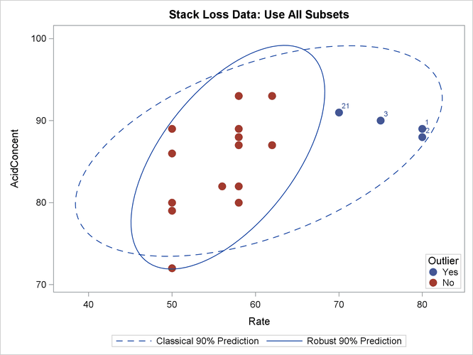
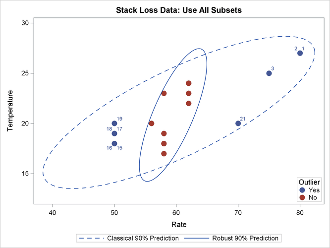
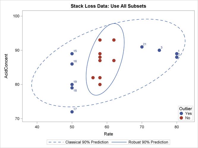
The following statements generate three bivariate scatter plots of the classical and robust tolerance ellipsoids. The plots are shown in Output 13.5.3, Output 13.5.4, and Output 13.5.5, one plot for each pair of variables.
optn = j(5,1,.); optn[5]= -1;
vnam = {"Rate", "Temperature", "AcidConcent"};
titl = "Stack Loss Data: Use All Subsets";
call MVEScatter(x, optn, 0.9, vnam, titl);
Output 13.5.3: Stack Loss Data: Rate versus Temperature (MVE)
Output 13.5.4: Stack Loss Data: Rate versus Acid Concentration (MVE)
Output 13.5.5: Stack Loss Data: Temperature versus Acid Concentration (MVE)
You can also use the MCD method for the stack loss data as follows:
optn = j(5,1,.);
optn[1]= 2;              /* print distances */
optn[2]= 1;              /* print covariance matrices */
optn[5]= -1 ;            /* nrep: use all subsets */

call mcd(sc, xmcd, dist, optn, x);
The optimization results are displayed in Output 13.5.6. The reweighted results are displayed in Output 13.5.7.
Output 13.5.6: MCD Results of Optimization
Output 13.5.7: Final Reweighted MCD Results
The MCD robust distances and outlying diagnostic are displayed in Output 13.5.8. MCD identifies more leverage points than MVE identifies.
Output 13.5.8: MCD Robust Distances
| Classical Distances and Robust (Rousseeuw) Distances | |||
|---|---|---|---|
| Unsquared Mahalanobis Distance and | |||
| Unsquared Rousseeuw Distance of Each Observation | |||
| N | Mahalanobis Distances | Robust Distances | Weight |
| 1 | 2.253603 | 12.173282 | 0 |
| 2 | 2.324745 | 12.255677 | 0 |
| 3 | 1.593712 | 9.263990 | 0 |
| 4 | 1.271898 | 1.401368 | 1.000000 |
| 5 | 0.303357 | 1.420020 | 1.000000 |
| 6 | 0.772895 | 1.291188 | 1.000000 |
| 7 | 1.852661 | 1.460370 | 1.000000 |
| 8 | 1.852661 | 1.460370 | 1.000000 |
| 9 | 1.360622 | 2.120590 | 1.000000 |
| 10 | 1.745997 | 1.809708 | 1.000000 |
| 11 | 1.465702 | 1.362278 | 1.000000 |
| 12 | 1.841504 | 1.667437 | 1.000000 |
| 13 | 1.482649 | 1.416724 | 1.000000 |
| 14 | 1.778785 | 1.988240 | 1.000000 |
| 15 | 1.690241 | 5.874858 | 0 |
| 16 | 1.291934 | 5.606157 | 0 |
| 17 | 2.700016 | 6.133319 | 0 |
| 18 | 1.503155 | 5.760432 | 0 |
| 19 | 1.593221 | 6.156248 | 0 |
| 20 | 0.807054 | 2.172300 | 1.000000 |
| 21 | 2.176761 | 7.622769 | 0 |
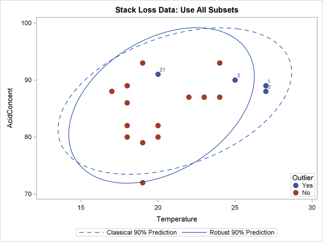
The following statements generate three bivariate scatter plots of the classical and robust tolerance ellipsoids:
optn = j(5,1,.); optn[5]= -1;
vnam = {"Rate", "Temperature", "AcidConcent"};
titl = "Stack Loss Data: Use All Subsets";
call MCDScatter(x, optn, 0.9, vnam, titl);
Output 13.5.9, Output 13.5.10, and Output 13.5.11 display these plots, one plot for each pair of variables:
Output 13.5.9: Stack Loss Data: Rate versus Temperature (MCD)
Output 13.5.10: Stack Loss Data: Rate versus Acid Concentration (MCD)
Output 13.5.11: Stack Loss Data: Temperature versus Acid Concentration (MCD)