Nonlinear Optimization Examples
Objective Function and Derivatives
The input argument fun refers to an IML module that specifies a function that returns f, a vector of length m for least squares subroutines or a scalar for other optimization subroutines. The returned f contains the values of the objective function (or the least squares functions) at the point x. Note that for least squares problems, you must specify the number of function values, m, with the first element of the opt argument to allocate memory for the return vector. All the modules that you can specify as input arguments ("fun," "grd," "hes," "jac," "nlc," "jacnlc," and "ptit") accept only a single input argument, x, which is the parameter vector. Using the GLOBAL clause, you can provide more input arguments for these modules. Refer to the section Numerical Considerations for an example.
All the optimization algorithms assume that f is continuous inside the feasible region. For nonlinearly constrained optimization, this is also required for points outside the feasible region. Sometimes the objective function cannot be computed for all points of the specified feasible region; for example, the function specification might contain the SQRT or LOG function, which cannot be evaluated for negative arguments. You must make sure that the function and derivatives of the starting point can be evaluated. There are two ways to prevent large steps into infeasible regions of the parameter space during the optimization process:
-
The preferred way is to restrict the parameter space by introducing more boundary and linear constraints. For example, the boundary constraint
 1E–10 prevents infeasible evaluations of
  . If the function module takes the square root or the log of an intermediate result, you can use nonlinear constraints to
try to avoid infeasible function evaluations. However, this might not ensure feasibility.
. If the function module takes the square root or the log of an intermediate result, you can use nonlinear constraints to
try to avoid infeasible function evaluations. However, this might not ensure feasibility.
-
Sometimes the preferred way is difficult to practice, in which case the function module can return a missing value. This can force the optimization algorithm to reduce the step length or the radius of the feasible region.
All the optimization techniques except the NLPNMS subroutine require continuous first-order derivatives of the objective function
f. The NLPTR, NLPNRA, and NLPNRR techniques also require continuous second-order derivatives. If you do not provide the derivatives
with the IML modules "grd," "hes," or "jac," they are automatically approximated by finite-difference formulas. Approximating first-order derivatives by finite differences
usually requires n additional calls of the function module. Approximating second-order derivatives by finite differences using only function
calls can be extremely computationally expensive. Hence, if you decide to use the NLPTR, NLPNRA, or NLPNRR subroutines, you
should specify at least analytical first-order derivatives. Then, approximating second-order derivatives by finite differences
requires only n or  additional calls of the function and gradient modules.
For all input and output arguments, the subroutines assume that
-
the number of parameters n corresponds to the number of columns. For example, x, the input argument to the modules, and g, the output argument returned by the "grd" module, are row vectors with n entries, and G, the Hessian matrix returned by the "hes" module, must be a symmetric
 matrix.
-
the number of functions, m, corresponds to the number of rows. For example, the vector f returned by the "fun" module must be a column vector with m entries, and in least squares problems, the Jacobian matrix
 returned by the "jac" module must be an
  matrix.
You can verify your analytical derivative specifications by computing finite-difference approximations of the derivatives of f with the NLPFDD subroutine. For most applications, the finite-difference approximations of the derivatives are very precise. Occasionally, difficult objective functions and zero x coordinates cause problems. You can use the par argument to specify the number of accurate digits in the evaluation of the objective function; this defines the step size h of the first- and second-order finite-difference formulas. See the section Finite-Difference Approximations of Derivatives.
Note: For some difficult applications, the finite-difference approximations of derivatives that are generated by default might not be precise enough to solve the optimization or least squares problem. In such cases, you might be able to specify better derivative approximations by using a better approximation formula. You can submit your own finite-difference approximations by using the IML module "grd," "hes," "jac," or "jacnlc." See Example 15.3 for an illustration.
In many applications, calculations used in the computation of f can help compute derivatives at the same point efficiently. You can save and reuse such calculations with the GLOBAL clause. As with many other optimization packages, the subroutines call the "grd," "hes," or "jac" modules only after a call of the "fun" module.
The following statements specify modules for the function, gradient, and Hessian matrix of the Rosenbrock problem:
proc iml;
start F_ROSEN(x);
   y1 = 10. * (x[2] - x[1] * x[1]);
   y2 = 1. - x[1];
   f  = .5 * (y1 * y1 + y2 * y2);
   return(f);
finish F_ROSEN;

start G_ROSEN(x);
   g = j(1,2,0.);
   g[1] = -200.*x[1]*(x[2]-x[1]*x[1]) - (1.-x[1]);
   g[2] =  100.*(x[2]-x[1]*x[1]);
   return(g);
finish G_ROSEN;

start H_ROSEN(x);
   h = j(2,2,0.);
   h[1,1] = -200.*(x[2] - 3.*x[1]*x[1]) + 1.;
   h[2,2] =  100.;
   h[1,2] = -200. * x[1];
   h[2,1] = h[1,2];
   return(h);
finish H_ROSEN;
Similarly, the following statements specify a module for the Rosenbrock function when considered as a least squares problem. They also specify the Jacobian matrix of the least squares functions.
start F_ROSEN_LS(x);
   y = j(1,2,0.);
   y[1] = 10. * (x[2] - x[1] * x[1]);
   y[2] = 1. - x[1];
  return(y);
finish F_ROSEN_LS;

start J_ROSEN(x);
   jac = j(2,2,0.);
   jac[1,1] = -20. * x[1]; jac[1,2] = 10.;
   jac[2,1] = -1.;         jac[2,2] =  0.;
   return(jac);
finish J_ROSEN;
Diagonal or Sparse Hessian Matrices
In the unconstrained or only boundary constrained case, the NLPNRA algorithm can take advantage of diagonal or sparse Hessian
matrices submitted by the "hes" module. If the Hessian matrix G of the objective function f has a large proportion of zeros, you can save computer time and memory by specifying a sparse Hessian of dimension  rather than a dense Hessian. Each of the
  rows
rows  of the matrix returned by the sparse Hessian module defines a nonzero element
  of the Hessian matrix. The row and column location is given by i and j, and g gives the nonzero value. During the optimization process, only the values g can be changed in each call of the Hessian module "hes;" the sparsity structure
  must be kept the same. That means that some of the values g can be zero for particular values of x. To allocate sufficient memory before the first call of the Hessian module, you must specify the number of rows, , by setting the ninth element of the opt argument.
Example 22 of Moré, Garbow, and Hillstrom (1981) illustrates the sparse Hessian module input. The objective function, which is the Extended Powell’s Singular Function, for
 is a least squares problem:
![\[ f(x) = \frac{1}{2} \{ f^2_1(x) + \cdots + f^2_ m(x) \} \]](images/imlug_nonlinearoptexpls0066.png)
with
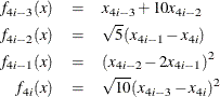
The function and gradient modules are as follows:
proc iml;
start f_nlp22(x);
   n=ncol(x);
   f = 0.;
   do i=1 to n-3 by 4;
      f1 = x[i] + 10. * x[i+1];
      r2 = x[i+2] - x[i+3];
      f2 = sqrt(5) * r2;
      r3 = x[i+1] - 2. * x[i+2];
      f3 = r3 * r3;
      r4 = x[i] - x[i+3];
      f4 = sqrt(10) * r4 * r4;
      f = f + f1 * f1 + r2 * f2 + f3 * f3 + r4 * r4 * f4;
   end;
   f = 0.5 * f;
   return(f);
finish f_nlp22;

start g_nlp22(x);
   n=ncol(x);
   g = j(1,n,0.);
      do i=1 to n-3 by 4;
         f1 = x[i] + 10. * x[i+1];
         f2 = sqrt(5) * (x[i+2] - x[i+3]);
         r3 = x[i+1] - 2. * x[i+2];
         f3 = r3 * r3;
         r4 = x[i] - x[i+3];
         f4 = sqrt(10) * r4 * r4;
         g[i]   = f1 + 2. * r4 * f4;
         g[i+1] = 10. * f1 + 2. * r3 * f3;
         g[i+2] = f2 - 4. * r3 * f3;
         g[i+3] = -f2 - 2. * r4 * f4;
      end;
      return(g);
finish g_nlp22;
You can specify the sparse Hessian with the following module:
start hs_nlp22(x);
   n=ncol(x);
   nnz = 8 * (n / 4);
   h = j(nnz,3,0.);
   j = 0;
   do i=1 to n-3 by 4;
      f1 = x[i] + 10. * x[i+1];
      f2 = sqrt(5) * (x[i+2] - x[i+3]);
      r3 = x[i+1] - 2. * x[i+2];
      f3 = r3 * r3;
      r4 = x[i] - x[i+3];
      f4 = sqrt(10) * r4 * r4;
      j= j + 1; h[j,1] = i; h[j,2] = i;
      h[j,3] = 1. + 4. * f4;
      h[j,3] = h[j,3] + 2. * f4;
      j= j+1; h[j,1] = i; h[j,2] = i+1;
      h[j,3] = 10.;
      j= j+1; h[j,1] = i; h[j,2] = i+3;
      h[j,3] = -4. * f4;
      h[j,3] = h[j,3] - 2. * f4;
      j= j+1; h[j,1] = i+1; h[j,2] = i+1;
      h[j,3] = 100. + 4. * f3;
      h[j,3] = h[j,3] + 2. * f3;
      j= j+1; h[j,1] = i+1; h[j,2] = i+2;
      h[j,3] = -8. * f3;
      h[j,3] = h[j,3] - 4. * f3;
      j= j+1; h[j,1] = i+2; h[j,2] = i+2;
      h[j,3] = 5. + 16. * f3;
      h[j,3] = h[j,3] + 8. * f3;
      j= j+1; h[j,1] = i+2; h[j,2] = i+3;
      h[j,3] = -5.;
      j= j+1; h[j,1] = i+3; h[j,2] = i+3;
      h[j,3] = 5. + 4. * f4;
      h[j,3] = h[j,3] + 2. * f4;
   end;
   return(h);
finish hs_nlp22;
n = 40;
x = j(1,n,0.);
do i=1 to n-3 by 4;
   x[i] = 3.; x[i+1] = -1.; x[i+3] = 1.;
end;
opt = j(1,11,.); opt[2]= 3; opt[9]= 8 * (n / 4);
call nlpnra(xr,rc,"f_nlp22",x,opt) grd="g_nlp22" hes="hs_nlp22";
Note: If the sparse form of Hessian defines a diagonal matrix (that is,  in all rows), the NLPNRA algorithm stores and processes a diagonal matrix G. If you do not specify any general linear constraints, the NLPNRA subroutine uses only order n memory.