Nonlinear Optimization Examples
Kuhn-Tucker Conditions
The nonlinear programming (NLP) problem with one objective function f and m constraint functions  , which are continuously differentiable, is defined as follows:
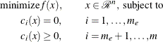
In the preceding notation, n is the dimension of the function  , and
, and  is the number of equality constraints. The linear combination of objective and constraint functions
![\[ L(x,\lambda ) = f(x) - \sum _{i=1}^ m \lambda _ i c_ i(x) \]](images/imlug_nonlinearoptexpls0046.png)
is the Lagrange function, and the coefficients  are the Lagrange multipliers.
If the functions f and are twice differentiable, the point  is an isolated local minimizer of the NLP problem, if there exists a vector
 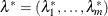 that meets the following conditions:
-
Kuhn-Tucker conditions
![\[ \begin{array}{ll} c_ i(x^*) = 0 , & i = 1, \ldots ,m_ e \\ c_ i(x^*) \ge 0 , ~ ~ \lambda _ i^* \ge 0, ~ ~ \lambda _ i^* c_ i(x^*) = 0 , & i = m_ e+1, \ldots ,m \\ \nabla _ x L(x^*,\lambda ^*) = 0 \end{array} \]](images/imlug_nonlinearoptexpls0049.png)
-
second-order condition
Each nonzero vector
 with
with
![\[ y^ T \nabla _ x c_ i(x^*) = 0 i = 1,\ldots ,m_ e ,\; \mbox{ and } \forall i\in {m_ e+1,\ldots ,m}; \lambda _ i^* > 0 \]](images/imlug_nonlinearoptexpls0051.png)
satisfies
![\[ y^ T \nabla _ x^2 L(x^*,\lambda ^*) y > 0 \]](images/imlug_nonlinearoptexpls0052.png)
In practice, you cannot expect the constraint functions  to vanish within machine precision, and determining the set of active constraints at the solution might not be simple.