General Statistics Examples

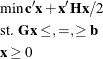
The following quadratic program can be solved by solving an equivalent linear complementarity problem when is positive semidefinite:

This approach is outlined in the discussion of the LCP subroutine .

The following routine solves the quadratic problem:

proc iml;
start qp( names, c, H, G, rel, b, activity);
   if min(eigval(h))<0 then do;
      error={'The minimum eigenvalue of the H matrix is negative.',
             'Thus it is not positive semidefinite.',
             'QP is terminating.'};
      print error;
      stop;
   end;
   nr=nrow(G);
   nc=ncol(G);

   /* Put in canonical form */
   rev = (rel='<=');
   adj = (-1 * rev) + ^rev;
   g = adj# G;
   b = adj # b;
   eq = ( rel = '='  );
   if max(eq)=1 then do;
      g = g // -(diag(eq)*G)[loc(eq),];
      b = b // -(diag(eq)*b)[loc(eq)];
   end;
   m = (h || -g`) // (g || j(nrow(g),nrow(g),0));
   q = c // -b;

   /* Solve the problem */
   call lcp(rc,w,z,M,q);

   /* Report the solution */
   print ({'*************Solution is optimal***************',
           '*********No solution possible******************',
           ' ', ' ', ' ',
           '**********Solution is numerically unstable*****',
           '***********Not enough memory*******************',
           '**********Number of iterations exceeded********'}[rc+1]);
   activity = z[1:nc];
   objval = c`*activity + activity`*H*activity/2;
   print objval[L='Objective Value'],
         activity[r=names L= 'Decision Variables'];
finish qp;

As an example, consider the following problem in portfolio selection. Models used in selecting investment portfolios include assessment of the proposed portfolio’s expected gain and its associated risk. One such model seeks to minimize the variance of the portfolio subject to a minimum expected gain. This can be modeled as a quadratic program in which the decision variables are the proportions to invest in each of the possible securities. The quadratic component of the objective function is the covariance of gain between the securities. The first constraint is a proportionality constraint; the second constraint gives the minimum acceptable expected gain.

The following data are used to illustrate the model and its solution:

c = { 0, 0, 0, 0 };
h = { 1003.1 4.3 6.3 5.9 ,
         4.3 2.2 2.1 3.9 ,
         6.3 2.1 3.5 4.8 ,
         5.9 3.9 4.8 10 };
g = {  1   1   1   1  ,
      .17 .11 .10 .18 };

/* constraints: proportions sum to 1; gain at least 10% */
b = { 1 , .10 };
rel = { '=', '>='};
names = 'Asset1':'Asset4';
run qp(names, c, h, g, rel, b, activity);

The results in Output 10.10.1 show that the minimum variance portfolio that achieves the 0.10 expected gain is composed of Asset2 and Asset3 in proportions of 0.933 and 0.067, respectively.