Time Series Analysis and Examples
In classical linear regression analysis, the underlying process can often be represented simply by an intercept and slope parameters. A time series can be modeled by a type of regression analysis.
The following subroutines and functions are supported:
- ARMACOV
-
computes an autocovariance sequence for an ARMA model.
- ARMALIK
-
computes the log likelihood and residuals for an ARMA model.
- ARMASIM
-
simulates an ARMA series.
The ARMACOV subroutine provides the pattern of the autocovariance function of AR, MA, and ARMA models and helps identify and fit a proper model.
The ARMALIK subroutine provides the log likelihood of an ARMA model and helps estimate the parameters of an ARMA regression model.
The ARMASIM function generates various time series from the underlying AR, MA, and ARMA models. Simulations of time series that have a known ARMA structure are often needed as part of other simulations or as learning data sets for developing time series analysis skills.
Consider a time series of length 100 from the ARMA(2,1) model
where the error series follows a normal distribution with mean 10 and standard deviation 2.
The following statements generate the ARMA(2,1) model:
proc iml;
/* ARMA(2,1) model */
phi = {1 -0.5 0.04};
theta = {1 0.25};
mu = 10;
sigma = 2;
nobs = 100;
seed = 3456;
lag = 10;
yt = armasim(phi, theta, mu, sigma, nobs, seed);
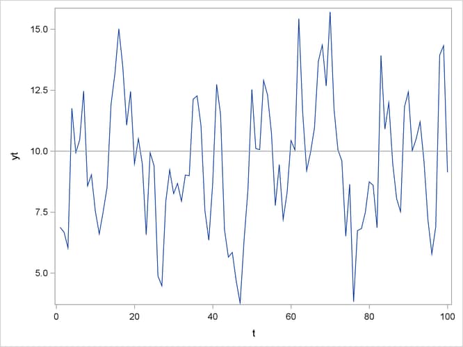
The ARMASIM function generates the data shown in Figure 13.1. The following statements compute 10 lags of the autocovariance function of the series. Figure 13.2 displays the autocovariance functions of the ARMA(2,1) model, the covariance functions of the moving-average term with lagged values of the process, and the autocovariance functions of the moving-average term.
call armacov(autocov, cross, convol, phi, theta, lag);
autocov = autocov`;  cross = cross`;  convol = convol`;
print autocov cross convol;
The following statements call the ARMALIK subroutine . The first column of Figure 13.3 contains the log-likelihood function, the estimate of the innovation variance, and the log of the determinant of the variance matrix. The next two columns display part of the standardized residuals and the scale factors that are used to standardize the residuals.
call armalik(lnl, resid, std, yt, phi, theta);
resid=resid[1:9];
std=std[1:9];
print lnl resid std;
Another example that uses the ARMACOV and ARMALIK subroutines is provided in Simulations of a Univariate ARMA Process.