Robust Regression Examples
A Hertzsprung-Russell diagram is a scatter plot that shows the relationship between the luminosity of stars and their effective
temperatures. The following data correspond to 47 stars of the CYG OB1 cluster in the direction of the constellation Cygnus
(Rousseeuw and Leroy, 1987; Humphreys, 1978; Vansina and De Greve, 1982). The regressor variable x (column 2) is the logarithm of the effective temperature at the surface of the star, and the response variable y (column 3) is the logarithm of its light intensity. This data set is remarkable in that it contains four substantial leverage
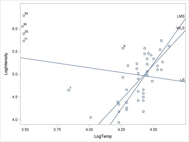
points (observations 11, 20, 30, and 34) that greatly affect the results of ![]() , and even
, and even ![]() , regression. The high leverage points, which represent giant stars, are shown in Output 12.1.2.
, regression. The high leverage points, which represent giant stars, are shown in Output 12.1.2.
The following SAS/IML statements define the data:
proc iml;
/* Hertzsprung-Russell Star Data */
/*  ObsNum LogTemp LogIntensity  */
hr = { 1  4.37  5.23,   2  4.56  5.74,   3  4.26  4.93,
       4  4.56  5.74,   5  4.30  5.19,   6  4.46  5.46,
       7  3.84  4.65,   8  4.57  5.27,   9  4.26  5.57,
      10  4.37  5.12,  11  3.49  5.73,  12  4.43  5.45,
      13  4.48  5.42,  14  4.01  4.05,  15  4.29  4.26,
      16  4.42  4.58,  17  4.23  3.94,  18  4.42  4.18,
      19  4.23  4.18,  20  3.49  5.89,  21  4.29  4.38,
      22  4.29  4.22,  23  4.42  4.42,  24  4.49  4.85,
      25  4.38  5.02,  26  4.42  4.66,  27  4.29  4.66,
      28  4.38  4.90,  29  4.22  4.39,  30  3.48  6.05,
      31  4.38  4.42,  32  4.56  5.10,  33  4.45  5.22,
      34  3.49  6.29,  35  4.23  4.34,  36  4.62  5.62,
      37  4.53  5.10,  38  4.45  5.22,  39  4.53  5.18,
      40  4.43  5.57,  41  4.38  4.62,  42  4.45  5.06,
      43  4.50  5.34,  44  4.45  5.34,  45  4.55  5.54,
      46  4.45  4.98,  47  4.42  4.50 } ;

x = hr[,2]; y = hr[,3];
You can call the LMS subroutine to carry out a least median squares regression analysis. In the following statements, the ODS SELECT statement limits the number of tables that are produced by the subroutine:
optn = j(9,1,.);
optn[2]= 1;    /* do not print residuals, diagnostics, or history */
optn[3]= 3;    /* compute LS, LMS, and weighted LS regression */

ods select LSEst EstCoeff RLSEstLMS;
call lms(sc, coef, wgt, optn, y, x);
ods select all;
Output 12.1.1 shows the parameter estimates for three regression models: the least squares (LS) model, the LMS model, and a weighted robust least squares (RLS) model.
The three regression lines are plotted in Output 12.1.2. The least squares line has a negative slope and a positive intercept. It is highly influenced by the four leverage points in the upper left portion of Output 12.1.2. In contrast, the LMS regression line (whose parameter estimates are shown in the "Estimated Coefficients" table) fits the bulk of the data and ignores the four leverage points.
Similarly, the weighted least squares line (in which the observations 7, 9, 11, 20, 30, and 34 are given zero weight) is less affected by the leverage points. The weights are determined by the size of the scaled residuals for the LMS regression.
In addition to the printed output, the LMS subroutine returns information about the fitted models in the sc, coef, and wgt matrices. The following statements display some of the values in the sc matrix. See Output 12.1.3.
r1 = {"Quantile", "Number of Subsets", "Number of Singular Subsets",
       "Number of Nonzero Weights", "Objective Function",
       "Preliminary Scale Estimate", "Final Scale Estimate",
       "Robust R Squared", "Asymptotic Consistency Factor"};
r2 = { "WLS Scale Estimate", "Weighted Sum of Squares",
       "Weighted R-squared", "F Statistic"};
sc1 = sc[1:9];
sc2 = sc[11:14];
print sc1[r=r1 L="LMS Information and Estimates"],
      sc2[r=r2 L="Weighted Least Squares"];
Output 12.1.3 shows summary statistics for the analysis. The analysis tries to minimize the hth ordered residual, where ![]() . The LMS algorithm randomly selects 1,081 subsets of three observations. Of these, 45 are singular. The subset that minimizes
the 25th ordered residual is found. Based on this subset, six observations are classified as outliers.
. The LMS algorithm randomly selects 1,081 subsets of three observations. Of these, 45 are singular. The subset that minimizes
the 25th ordered residual is found. Based on this subset, six observations are classified as outliers.
The coef matrix contains as many columns as there are regressor variables. Rows of the coef matrix contain parameter estimates and related statistics. The wgt matrix contains as many columns as there are observations. Rows of the wgt matrix contain an indicator variable for outliers and residuals for the robust regression.
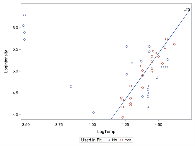
An alternative to LMS regression is least trimmed squares (LTS) regression. The LTS subroutine implements the FAST-LTS regression algorithm, which improves the Rousseeuw and Leroy (1987) algorithm (called V7 LTS in this chapter) by using techniques called "selective iteration" and "nested extensions." These techniques are used in the C-steps of the algorithm. See Rousseeuw and Van Driessen (2000) for details. The FAST-LTS algorithm significantly improves the speed of computation.
The LTS subroutine performs least trimmed squares (LTS) robust regression by minimizing the sum of the h smallest squared residuals. The following statements compute the LTS regression for the Hertzsprung-Russell star data:
optn = j(9,1,.);
optn[2]= 3;    /* print a maximum amount of information */
optn[3]= 3;    /* compute LS, LTS, and weighted LS regression */

ods select BestHalf EstCoeff;
call lts(sc, coef, wgt, optn, y, x);
ods select all;
The line of best fit for the LTS regression has slope 4.23 and intercept ![]() as shown in the "Estimated Coefficients" table in Output 12.1.4. This is a steeper line than for the LMS regression, which is shown in Output 12.1.1.
as shown in the "Estimated Coefficients" table in Output 12.1.4. This is a steeper line than for the LMS regression, which is shown in Output 12.1.1.
Output 12.1.5 shows the best subset of observations for the Hertzsprung-Russell data. There are ![]() observations in Output 12.1.5.
observations in Output 12.1.5.
Output 12.1.6 shows the geometric meaning of the best subset. In the graph, the selected observations determine the regression line. The observations that are not contained in the best subset are not used to fit the regression line.