Language Reference
CALL LCP (rc, w, z, m, q <, epsilon> );
The LCP subroutine solves the linear complementarity problem:
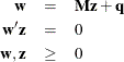
That is, given a matrix ![]() and a vector
and a vector ![]() , the LCP subroutine computes orthogonal, nonnegative vectors
, the LCP subroutine computes orthogonal, nonnegative vectors ![]() and
and ![]() which satisfy the previous equations.
which satisfy the previous equations.
The input arguments to the LCP subroutine are as follows:
- m
-
is an
 matrix.
- q
-
is an
 matrix.
- epsilon
-
is a scalar that defines virtual zero. The default value of epsilon is 1E
 8.
8.
The LCP subroutine returns the following matrices:
- rc
-
returns one of the following scalar return codes:
rc
Termination
0
A solution is found.
1
No solution is possible.
5
The solution is numerically unstable.
6
The subroutine could not obtain enough memory.
- w
-
returns an m-element column vector
- z
-
returns an m-element column vector
The following statements give a simple example:
q = {1, 1};
m = {1 0,
     0 1};
call lcp(rc, w, z, m, q);
print rc, w, z;
The next example shows the relationship between quadratic programming and the linear complementarity problem. Consider the linearly constrained quadratic program:
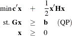
If ![]() is positive semidefinite, then a solution to the Kuhn-Tucker conditions solves QP. The Kuhn-Tucker conditions for QP are
is positive semidefinite, then a solution to the Kuhn-Tucker conditions solves QP. The Kuhn-Tucker conditions for QP are
![\begin{eqnarray*} \mb{c} + \mb{Hx} & = & \mu + \mb{G}^{\prime } { \lambda } \\ \lambda ^{\prime } (\mb{Gx}- \mb{b}) & = & 0 \\ {\mu }^{\prime } \mb{x} & = & 0 \\ \mb{Gx} & \geq & \mb{b} \\[0.10in] {x, \mu ,\lambda } & \geq & 0 ~ \end{eqnarray*}](images/imlug_langref0700.png)
In the linear complementarity problem, let
![\begin{eqnarray*} \mb{M} & = & \left[ \begin{array}{cc} H & -G^{\prime } \\ G & 0 \\ \end{array} \right] \\ \mb{w}^{\prime } & = & ({\mu }^{\prime }\mb{s}^{\prime }) \\ \mb{z}^{\prime } & = & (\mb{x}^{\prime }{ \lambda }^{\prime }) \\ \mb{q}^{\prime } & = & (\mb{c}^{\prime } - \mb{b}) ~ \end{eqnarray*}](images/imlug_langref0701.png)
Then the Kuhn-Tucker conditions are expressed as finding ![]() and
and ![]() that satisfy
that satisfy

From the solution ![]() and
and ![]() to this linear complementarity problem, the solution to QP is obtained; namely,
to this linear complementarity problem, the solution to QP is obtained; namely, ![]() is the primal structural variable,
is the primal structural variable, ![]() the surpluses, and
the surpluses, and ![]() and
and ![]() are the dual variables. Consider a quadratic program with the following data:
are the dual variables. Consider a quadratic program with the following data:
![\begin{eqnarray*} \mb{C}^{\prime } & = & (1 2 4 5) ~ ~ ~ ~ ~ \mb{B}^{\prime } = ( 1 1 ) \\[0.10in] \mb{H} & = & \left[ \begin{array}{rrrr} 100 & 10 & 1 & 0 \\ 10 & 100 & 10 & 1 \\ 1 & 10 & 100 & 10 \\ 0 & 1 & 10 & 100 \end{array} \right] \\[0.10in] \mb{G} & = & \left[ \begin{array}{rrrr} 1 & 2 & 3 & 4 \\ 10 & 20 & 30 & 40 \end{array} \right] \\ \end{eqnarray*}](images/imlug_langref0706.png)
This problem is solved by using the LCP subroutine as follows:
/*---- Data for the Quadratic Program -----*/
c = {1, 2, 3, 4};
h = {100 10 1 0, 10 100 10 1, 1 10 100 10, 0 1 10 100};
g = {1 2 3 4, 10 20 30 40};
b = {1, 1};

/*----- Express the Kuhn-Tucker Conditions as an LCP ----*/
m = h || -g`;
m = m // (g || j(nrow(g),nrow(g),0));
q = c // -b;

/*----- Solve for a Kuhn-Tucker Point --------*/
call lcp(rc, w, z, m, q);

/*------ Extract the Solution to the Quadratic Program ----*/
x = z[1:nrow(h)];
print rc x;