Example: Solving a System of Linear Equations :: SAS/IML(R) 13.1 User's Guide

Example: Solving a System of Linear Equations

Because the syntax of the SAS/IML language is similar to the notation used in linear algebra, it is often possible to directly translate mathematical methods from matrix-algebraic expressions into executable SAS/IML statements. For example, consider the problem of solving three simultaneous equations:

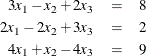
$\begin{eqnarray*} 3x_1 - x_2 + 2x_3 & = & 8 \\ 2x_1 - 2x_2 + 3x_3 & = & 2 \\ 4x_1 + x_2 - 4x_3 & = & 9 \\ \end{eqnarray*}$

These equations can be written in matrix form as

$\left[ \begin{array}{rrr} 3 & -1 & 2 \\ 2 & -2 & 3 \\ 4 & 1 & -4 \\ \end{array} \right] \left[ \begin{array}{c} x_1 \\ x_2 \\ x_3 \\ \end{array} \right] ~ = ~ \left[ \begin{array}{c} 8 \\ 2 \\ 9 \\ \end{array} \right]$

and can be expressed symbolically as

$\mb {Ax} = \mb {c}$

where $\mb {A}$ is the matrix of coefficients for the linear system. Because $\mb {A}$ is nonsingular, the system has a solution given by

$\mb {x} = \mb {A}^{-1}\mb {c} ~$

This example solves this linear system of equations.

Define the matrices $\mb {A}$ and $\mb {c}$ . Both of these matrices are input as matrix literals; that is, you type the row and column values as discussed in Chapter 3: Understanding the SAS/IML Language.
```
proc iml;
a = {3  -1  2,
     2  -2  3,
     4   1 -4};
c = {8, 2, 9};
```

Solve the equation by using the built-in INV function and the matrix multiplication operator. The INV function returns the inverse of a square matrix and * is the operator for matrix multiplication. Consequently, the solution is computed as follows:

x = inv(a) * c;
print x;

Figure 4.1: The Solution of a Linear System of Equations

x
3
5
2

Equivalently, you can solve the linear system by using the more efficient SOLVE function, as shown in the following statement:
```
x = solve(a, c);
```

After SAS/IML executes the statements, the rows of the vector x contain the $x_1, x_2$ , and $x_3$ values that solve the linear system.

You can end PROC IML by using the QUIT statement:

quit;