Getting Started :: SAS/IML(R) 13.1 User's Guide

Getting Started

The fractional differencing enables the degree of differencing $d$ to take any real value rather than being restricted to integer values. The fractionally differenced processes are capable of modeling long-term persistence. The process

$(1-B)^ dy_{t} = {\epsilon }_ t$

is known as a fractional Gaussian noise process or an ARFIMA( $0,d,0$ ) process, where $d\in (-1,1) \textbf{a}ckslash \{ 0\}$ , $\epsilon _ t$ is a white noise process with mean zero and variance $\sigma _{\epsilon }^2$ , and $B$ is the backshift operator such that $B^ j\mb {y}_{t}=\mb {y}_{t-j}$ . The extension of an ARFIMA( $0,d,0$ ) model combines fractional differencing with an ARMA( $p,q$ ) model, known as an ARFIMA( $p,d,q$ ) model.

Consider an ARFIMA( $0,0.4,0$ ) represented as $(1-B)^{0.4}y_{t} = {\epsilon }_ t$ where $\epsilon _ t \sim iid ~ N(0, 2)$ . With the following statements you can

generate the simulated 300 observations data
obtain the fractionally differenced data
compute the autocovariance function
compute the log-likelihood function
fit a fractionally integrated time series model to the data

proc iml;
/* ARFIMA(0,0.4,0) */
lag = (0:12)`;
call farmacov(autocov_D_IS_04, 0.4);
call farmacov(D_IS_005, 0.05);
print lag autocov_D_IS_04 D_IS_005;
d = 0.4;
call farmasim(yt, d) n=300 sigma=2 seed=5345;
call fdif(zt, yt, d);
*print zt;
call farmalik(lnl, yt, d);
print lnl;
call farmafit(d, ar, ma, sigma, yt);
print d sigma;

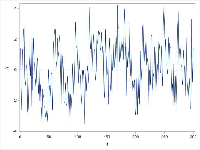
Output 13.21: Plot of Generated ARFIMA(0,0.4,0) Process (FARMASIM)

The FARMASIM function generates the data shown in Output 13.21.

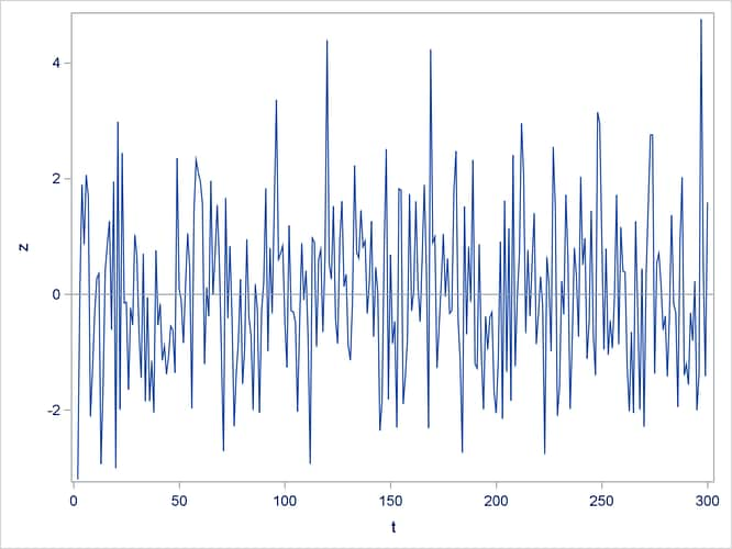
Output 13.22: Plot of Fractionally Differenced Process (FDIF)

The FDIF function creates the fractionally differenced process. Output 13.22 shows a white noise series.

Output 13.23: Autocovariance Functions of ARFIMA(0,0.4,0) and ARFIMA(0,0.05,0) Models (FARMACOV)

lag	autocov_D_IS_04	D_IS_005
0	2.0700983	1.0044485
1	1.3800656	0.0528657
2	1.2075574	0.0284662
3	1.1146683	0.0197816
4	1.0527423	0.0152744
5	1.0069709	0.0124972
6	0.9710077	0.0106069
7	0.9415832	0.0092333
8	0.9168047	0.008188
9	0.8954836	0.0073647
10	0.8768277	0.0066985
11	0.8602838	0.006148
12	0.8454513	0.0056849

The first column is the autocovariance function of the ARFIMA(0,0.4,0) model, and the second column is the autocovariance function of the ARFIMA(0,0.05,0) model. The first column decays to zero more slowly than the second column.

Output 13.24: Log-Likelihood Function of ARFIMA(0,0.4,0) Model (FARMALIK)

lnl
-101.0599
.
.

The first row value is the log-likelihood function of the ARFIMA(0,0.4,0) model. Because the default option of the estimates method is the conditional sum of squares, the last two rows of Output 13.24 contain missing values.

Output 13.25: Parameter Estimation of ARFIMA(0,0.4,0) Model (FARMAFIT)

d	sigma
0.386507	1.9610507

The final estimates of the parameters are $d=0.387$ and $\sigma ^2=1.96$ , while the true values of the data generating process are $d=0.4$ and $\sigma ^2=2$ .