VARMASIM Call :: SAS/IML(R) 12.3 User's Guide

VARMASIM Call

CALL VARMASIM (series, phi, theta, mu, sigma, n <*>, p <*>, q <*>, initial <*>, seed ) ;

The VARMASIM subroutine generates a VARMA(,) time series.

The input arguments to the VARMASIM subroutine are as follows:

phi

specifies a $km_ p \times k$ matrix that contains the autoregressive coefficient matrices, where is the number of the elements in the subset of the AR order and $k\geq 2$ is the number of variables. You must specify either phi or theta.

theta

specifies a $km_ q \times k$ matrix that contains the moving average coefficient matrices, where is the number of the elements in the subset of the MA order. You must specify either phi or theta.

mu

specifies a $k \times 1$ (or $1 \times k$ ) mean vector of the series. If mu is not specified, a zero vector is used.

sigma

specifies a $k \times k$ covariance matrix of the innovation series. If sigma is not specified, an identity matrix is used.

n

specifies the length of the series. If n is not specified, is used.

p

specifies the subset of the AR order. See the VARMACOV subroutine.

q

specifies the subset of the MA order. See the VARMACOV subroutine.

initial

specifies the initial values of random variables. If , then $\mb {y}_{-p+1},\ldots ,\mb {y}_{0}$ and $\bm {\epsilon }_{-q+1},\ldots , \bm {\epsilon }_{0}$ all take the same value . If the initial option is not specified, the initial values are estimated for the stationary vector time series; the initial values are assumed as zero for the nonstationary vector time series.

seed

is a scalar that contains the random number seed. At the first execution of the subroutine, the seed variable is used as follows:

If seed > 0, the input seed is used for generating the series.

If seed = 0, the system clock is used to generate the seed.

If seed < 0, the value () $\times$ (seed) is used for generating the series.

If the seed is not supplied, the system clock is used to generate the seed.

On subsequent calls of the subroutine in the DO loop like environment the seed variable is used as follows: If seed > 0, the seed remains unchanged. In other cases, after each execution of the subroutine, the current seed is updated internally.

The VARMASIM subroutine returns the following value:

series: is an $n\times k$ matrix that contains the generated VARMA() time series. When either the initial option is specified or zero initial values are used, these initial values are not included in series.

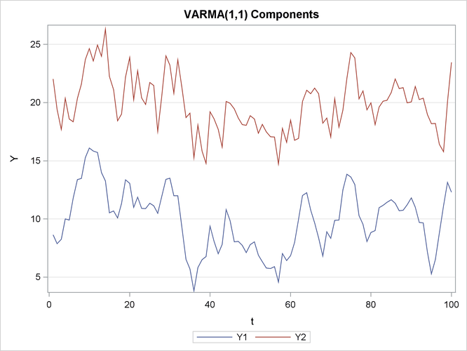
Consider the following bivariate () stationary VARMA(1,1) time series:

$\mb {y}_ t - \bm {\mu } = \Phi ( \mb {y}_{t-1} - \bm {\mu } ) + \bm {\epsilon }_ t - \Theta \bm {\epsilon }_{t-1}$

$\Phi =\left[\begin{matrix} 1.2 & -0.5 \cr 0.6 & 0.3 \cr \end{matrix}\right] ~ ~ \Theta =\left[\begin{matrix} -0.6 & 0.3 \cr 0.3 & 0.6 \cr \end{matrix}\right] ~ ~ \bm {\mu }=\left[\begin{matrix} 10 \cr 20 \cr \end{matrix}\right] ~ ~ \Sigma =\left[\begin{matrix} 1.0 & 0.5 \cr 0.5 & 1.25 \cr \end{matrix}\right]$

To generate this series, you can use the following statements:

phi  = { 1.2 -0.5, 0.6 0.3 };
theta= {-0.6  0.3, 0.3 0.6 };
mu   = { 10, 20 };
sigma= { 1.0  0.5, 0.5 1.25};
call varmasim(yt, phi, theta, mu, sigma, 100) seed=123;

Each column of the matrix yt is plotted in Figure 23.370. The first series oscillates about a mean value of 10; the second series oscillates about a mean value of 20.

Figure 23.370: Time Series Components

You can also simulate a nonstationary VARMA(1,1) time series with the same $\bm {\mu }$ , $\Sigma$ , and $\Theta$ as in the previous example and with the following AR coefficient:

$\Phi =\left[\begin{matrix} 1.0 & 0 \cr 0 & 0.3 \cr \end{matrix}\right]$

To generate this series, you can use the following statements:

phi  = { 1.0 0.0, 0.0 0.3 };
call varmasim(yt, phi, theta, mu, sigma, 100) initial=3 seed=123;