The technique of estimating parameters in linear models by using the notion of regression quantiles is a generalization of
the LAE or LAV least absolute value estimation technique. For a given quantile ![]() , the estimate
, the estimate ![]() of
of ![]() in the model
in the model
is the value of ![]() that minimizes
that minimizes
where ![]() and
and ![]() . For
. For ![]() , the solution
, the solution ![]() is identical to the estimates produced by the LAE. The following routine finds this estimate by using linear programming.
is identical to the estimates produced by the LAE. The following routine finds this estimate by using linear programming.
   /* Routine to find regression quantiles                    */
   /* yname:    name of dependent variable                    */
   /* y:        dependent variable                            */
   /* xname:    names of independent variables                */
   /* X:        independent variables                         */
   /* b:        estimates                                     */
   /* predict:  predicted values                              */
   /* error:    difference of y and predicted.                */
   /* q:        quantile                                      */
   /*                                                         */
   /* notes:    This subroutine finds the estimates b         */
   /* that minimize                                           */
   /*                                                         */
   /*           q * (y - Xb) * e  + (1-q) * (y - Xb) * ^e     */
   /*                                                         */
   /* where e = ( Xb <= y ).                                  */
   /*                                                         */
   /* This subroutine follows the approach given in:          */
   /*                                                         */
   /* Koenker, R. and G. Bassett (1978). Regression           */
   /* quantiles. Econometrica. Vol. 46. No. 1. 33-50.         */
   /*                                                         */
   /* Basssett, G. and R. Koenker (1982). An empirical        */
   /* quantile function for linear models with iid errors.    */
   /* JASA. Vol. 77. No. 378. 407-415.                        */
   /*                                                         */
   /* When q = .5 this is equivalent to minimizing the sum    */
   /* of the absolute deviations, which is also known as      */
   /* L1 regression.  Note that for L1 regression, a faster   */
   /* and more accurate algorithm is available in the SAS/IML */
   /* routine LAV, which is based on the approach given in:   */
   /*                                                         */
   /* Madsen, K. and Nielsen, H. B. (1993). A finite          */
   /* smoothing algorithm for linear L1 estimation.           */
   /* SIAM J. Optimization, Vol. 3. 223-235.                  */
   /*---------------------------------------------------------*/
   start rq( yname, y, xname, X, b, predict, error, q);
      bound=1.0e10;
      coef = X`;
      m = nrow(coef);
      n = ncol(coef);
   /*-----------------build rhs and bounds--------------------*/
      e  = repeat(1,1,n)`;
      r  =  {0 0} || ((1-q)*coef*e)`;
      sign = repeat(1,1,m);

      do i=1 to m;
         if r[2+i] < 0 then do;
            sign[i]   = -1;
            r[2+i]    = -r[2+i];
           coef[i,]  = -coef[i,];
         end;
      end;

   l  = repeat(0,1,n) || repeat(0,1,m)  || -bound || -bound ;
   u  = repeat(1,1,n) || repeat(.,1,m)  ||   { . . }  ;

   /*-------------build coefficient matrix and basis----------*/
    a  = (        y`     || repeat(0,1,m)  ||   { -1 0 }   ) //
         ( repeat(0,1,n) || repeat(-1,1,m) ||   { 0 -1 }   ) //
         (      coef     ||     I(m)       || repeat(0,m,2)) ;
    basis = n+m+2 - (0:n+m+1);

   /*----------------find a feasible solution-----------------*/
   call lp(rc,p,d,a,r,,u,l,basis);

   /*----------------find the optimal solution----------------*/
   l  = repeat(0,1,n) || repeat(0,1,m)  || -bound || {0} ;
   u  = repeat(1,1,n) || repeat(0,1,m)  ||   { . 0 }  ;
   call lp(rc,p,d,a,r,n+m+1,u,l,basis);

   /*---------------- report the solution-----------------------*/
   variable = xname`; b=d[3:m+2];
   do i=1 to m;
      b[i] =  b[i] * sign[i];
   end;
   predict = X*b;
   error = y - predict;
   wsum  = sum ( choose(error<0 , (q-1)*error , q*error) );

   print ,,'Regression Quantile Estimation' ,
           'Dependent Variable: ' yname ,
           'Regression Quantile: ' q ,
           'Number of Observations: ' n ,
           'Sum of Weighted Absolute Errors: ' wsum ,
            variable b,
            X y predict error;
   finish rq;
The following example uses data on the United States population from 1790 to 1970:
   z = { 3.929 1790 ,
         5.308 1800 ,
         7.239 1810 ,
         9.638 1820 ,
        12.866 1830 ,
        17.069 1840 ,
        23.191 1850 ,
        31.443 1860 ,
        39.818 1870 ,
        50.155 1880 ,
        62.947 1890 ,
        75.994 1900 ,
        91.972 1910 ,
       105.710 1920 ,
       122.775 1930 ,
       131.669 1940 ,
       151.325 1950 ,
       179.323 1960 ,
       203.211 1970 };

   y=z[,1];
   x=repeat(1,19,1)||z[,2]||z[,2]##2;
   run rq('pop',y,{'intercpt' 'year' 'yearsq'},x,b1,pred,resid,.5);
The results are shown in Output 9.11.1.
Output 9.11.1: Regression Quantiles: Results
| Regression Quantile Estimation |
| yname | |
|---|---|
| Dependent Variable: | pop |
| q | |
|---|---|
| Regression Quantile: | 0.5 |
| n | |
|---|---|
| Number of Observations: | 19 |
| wsum | |
|---|---|
| Sum of Weighted Absolute Errors: | 14.826429 |
| variable | b |
|---|---|
| intercpt | 21132.758 |
| year | -23.52574 |
| yearsq | 0.006549 |
| X | y | predict | error | ||
|---|---|---|---|---|---|
| 1 | 1790 | 3204100 | 3.929 | 5.4549176 | -1.525918 |
| 1 | 1800 | 3240000 | 5.308 | 5.308 | -4.54E-12 |
| 1 | 1810 | 3276100 | 7.239 | 6.4708902 | 0.7681098 |
| 1 | 1820 | 3312400 | 9.638 | 8.9435882 | 0.6944118 |
| 1 | 1830 | 3348900 | 12.866 | 12.726094 | 0.1399059 |
| 1 | 1840 | 3385600 | 17.069 | 17.818408 | -0.749408 |
| 1 | 1850 | 3422500 | 23.191 | 24.220529 | -1.029529 |
| 1 | 1860 | 3459600 | 31.443 | 31.932459 | -0.489459 |
| 1 | 1870 | 3496900 | 39.818 | 40.954196 | -1.136196 |
| 1 | 1880 | 3534400 | 50.155 | 51.285741 | -1.130741 |
| 1 | 1890 | 3572100 | 62.947 | 62.927094 | 0.0199059 |
| 1 | 1900 | 3610000 | 75.994 | 75.878255 | 0.1157451 |
| 1 | 1910 | 3648100 | 91.972 | 90.139224 | 1.8327765 |
| 1 | 1920 | 3686400 | 105.71 | 105.71 | 8.669E-13 |
| 1 | 1930 | 3724900 | 122.775 | 122.59058 | 0.1844157 |
| 1 | 1940 | 3763600 | 131.669 | 140.78098 | -9.111976 |
| 1 | 1950 | 3802500 | 151.325 | 160.28118 | -8.956176 |
| 1 | 1960 | 3841600 | 179.323 | 181.09118 | -1.768184 |
| 1 | 1970 | 3880900 | 203.211 | 203.211 | -2.96E-12 |
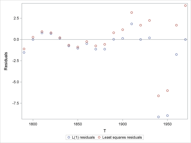
The L1 norm (when ![]() ) tends to cause the fit to be better at more points at the expense of causing some points to fit worse, as shown by the following
plot, which compares the L1 residuals with the least squares residuals.
) tends to cause the fit to be better at more points at the expense of causing some points to fit worse, as shown by the following
plot, which compares the L1 residuals with the least squares residuals.
When ![]() , the results of this module can be compared with the results of the LAV routine, as follows:
, the results of this module can be compared with the results of the LAV routine, as follows:
   b0 = {1 1 1};              /* initial value             */
   optn = j(4,1,.);           /* options vector            */

   optn[1]= .;                /* gamma default             */
   optn[2]= 5;                /* print all                 */
   optn[3]= 0;                /* McKean-Schradar variance  */
   optn[4]= 1;                /* convergence test          */

   call LAV(rc, xr, x, y, b0, optn);