Overview

SAS/IML has four subroutines that can be used for outlier detection and robust regression. The Least Median of Squares (LMS) and Least Trimmed Squares (LTS) subroutines perform robust regression (sometimes called resistant regression). These subroutines are able to detect outliers and perform a least-squares regression on the remaining observations. The Minimum Volume Ellipsoid Estimation (MVE) and Minimum Covariance Determinant Estimation (MCD) subroutines can be used to find a robust location and a robust covariance matrix that can be used for constructing confidence regions, detecting multivariate outliers and leverage points, and conducting robust canonical correlation and principal component analysis.

The LMS, LTS, MVE, and MCD methods were developed by Rousseeuw (1984) and Rousseeuw and Leroy (1987). All of these methods have the high breakdown value property. Roughly speaking, the breakdown value is a measure of the proportion of contamination that a procedure can withstand and still maintain its robustness.

The algorithm used in the LMS subroutine is based on the PROGRESS program of Rousseeuw and Hubert (1996), which is an updated version of Rousseeuw and Leroy (1987). In the special case of regression through the origin with a single regressor, Barreto and Maharry (2006) show that the PROGRESS algorithm does not, in general, find the slope that yields the least median of squares. Starting with release 9.2, the LMS subroutine uses the algorithm of Barreto and Maharry (2006) to obtain the correct LMS slope in the case of regression through the origin with a single regressor. In this case, inputs to the LMS subroutine specific to the PROGRESS algorithm are ignored and output specific to the PROGRESS algorithm is suppressed.

The algorithm used in the LTS subroutine is based on the algorithm FAST-LTS of Rousseeuw and Van Driessen (2000). The MCD algorithm is based on the FAST-MCD algorithm given by Rousseeuw and Van Driessen (1999), which is similar to the FAST-LTS algorithm. The MVE algorithm is based on the algorithm used in the MINVOL program by Rousseeuw (1984). LTS estimation has higher statistical efficiency than LMS estimation. With the FAST-LTS algorithm, LTS is also faster than LMS for large data sets. Similarly, MCD is faster than MVE for large data sets.

Besides LTS estimation and LMS estimation, there are other methods for robust regression and outlier detection. You can refer to a comprehensive procedure, PROC ROBUSTREG, in SAS/STAT. A summary of these robust tools in SAS can be found in Chen (2002).

The four SAS/IML subroutines are designed for the following:

• LMS: minimizing the th ordered squared residual

• LTS: minimizing the sum of the smallest squared residuals

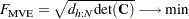
• MCD: minimizing the determinant of the covariance of points

• MVE: minimizing the volume of an ellipsoid that contains points

where is defined in the range

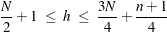In the preceding equation, is the number of observations and is the number of regressors.¹ The value of determines the breakdown value, which is "the smallest fraction of contamination that can cause the estimator to take on values arbitrarily far from " (Rousseeuw and Leroy; 1987). Here, denotes an estimator and applies to a sample .

For each parameter vector , the residual of observation is . You then denote the ordered, squared residuals as

The objective functions for the LMS, LTS, MCD, and MVE optimization problems are defined as follows:

• LMS, the objective function for the LMS optimization problem is the th ordered squared residual,

  Note that, for , the th quantile is the median of the squared residuals. The default in PROGRESS is , which yields the breakdown value (where denotes the integer part of ).

• LTS, the objective function for the LTS optimization problem is the sum of the smallest ordered squared residuals,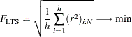

• MCD, the objective function for the MCD optimization problem is based on the determinant of the covariance of the selected points,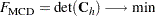

  where is the covariance matrix of the selected points.

• MVE, the objective function for the MVE optimization problem is based on the th quantile of the Mahalanobis-type distances ,

  subject to , where is the scatter matrix estimate, and the Mahalanobis-type distances are computed as

  where is the location estimate.

Because of the nonsmooth form of these objective functions, the estimates cannot be obtained with traditional optimization algorithms. For LMS and LTS, the algorithm, as in the PROGRESS program, selects a number of subsets of observations out of the given observations, evaluates the objective function, and saves the subset with the lowest objective function. As long as the problem size enables you to evaluate all such subsets, the result is a global optimum. If computing time does not permit you to evaluate all the different subsets, a random collection of subsets is evaluated. In such a case, you might not obtain the global optimum.

Note that the LMS, LTS, MCD, and MVE subroutines are executed only when the number of observations is more than twice the number of explanatory variables (including the intercept)—that is, if .