| KALCVF Call |
The KALCVF subroutine computes the one-step prediction  and the filtered estimate
  , in addition to their covariance matrices. The call uses forward recursions, and you can also use it to obtain
  -step estimates.
The input arguments to the KALCVF subroutine are as follows:
- data
is a
 matrix that contains data
  .
. - lead
is the number of steps to forecast after the end of the data.
- a
is an
 vector for a time-invariant input vector in the transition equation, or a
  vector that contains input vectors in the transition equation.
 - f
is an
 matrix for a time-invariant transition matrix in the transition equation, or a
  matrix that contains transition matrices in the transition equation.
 - b
is an
 vector for a time-invariant input vector in the measurement equation, or a
  vector that contains input vectors in the measurement equation.
 - h
is an
 matrix for a time-invariant measurement matrix in the measurement equation, or a
  matrix that contains measurement matrices in the measurement equation.
 - var
is an
 matrix for a time-invariant variance matrix for the error in the transition equation and the error in the measurement equation, or a
  matrix that contains variance matrices for the error in the transition equation and the error in the measurement equation—that is,
  .
. - z0
is an optional
 initial state vector
  .
. - vz0
is an optional
covariance matrix of an initial state vector  .
.
The KALCVF call returns the following values:
- pred
is a
 matrix that contains one-step predicted state vectors
  .
. - vpred
is a
matrix that contains mean square errors of predicted state vectors  .
. - filt
is a
 matrix that contains filtered state vectors
  .
. - vfilt
is a
 matrix that contains mean square errors of filtered state vectors
  .
.
The KALCVF call computes the conditional expectation of the state vector  given the observations, assuming that the mean and the variance of the initial state vector are known. The filtered value is the conditional expectation of the state vector given the observations up to time
  . For -step forecasting where
  , the conditional expectation at time
  is computed given observations up to . For notation,
  and
and  are variances of
  and
and  , respectively, and
  is a covariance of and , and
  stands for the generalized inverse of
  . The filtered value and its covariance matrix are denoted and
  , respectively. For ,
  and
and  stand for the -step forecast of
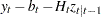
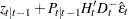
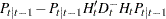
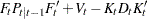
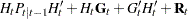
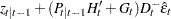
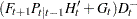
  and its mean square error. The Kalman filtering algorithm for one-step prediction and filtering is given as follows:
 |
 |
 |
|||
 |
|
 |
|||
 |
|
 |
|||
 |
|
 |
|||
 |
|
 |
|||
 |
|
 |
|||
 |
|
 |
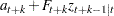
And for -step forecasting for  ,
,
 |
|
 |
|||
 |
|
 |
When you use the alternative transition equation
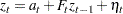 |
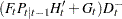
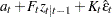
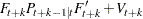
the forward recursion algorithm is written
|
|
|
|||
|
|
 |
|||
|
|
 |
|||
|
|
 |
|||
|
|
 |
|||
|
|
 |
|||
|
|
 |
And for -step forecasting  ,
,
|
|
 |
|||
|
|
 |
You can use the KALCVF call when you specify the alternative transition equation and  .
.
The initial state vector and its covariance matrix of the time-invariant Kalman filters are computed under the stationarity condition
 |
|
 |
|||
 |
|
 |
where  and
and  are the time-invariant transition matrix and the covariance matrix of transition equation noise, and vec
 is an
is an  column vector that is constructed by the stacking
  columns of matrix . Note that all eigenvalues of the matrix are inside the unit circle when the SSM is stationary. When the preceding formula cannot be applied, the initial state vector estimate
  is set to
  and its covariance matrix is given by
  I. Optionally, you can specify initial values.
The KALCVF call accepts missing values in observations. If there is a missing observation, the filtered state vector for the missing observation is given by the one-step forecast.
The following program gives an example of the KALCVF call:
q = 2;
p = 2;
n = 10;
lead = 3;
total = n + lead;

seed = 25735;
x = round(10*normal(j(n, p, seed)))/10;
f = round(10*normal(j(q*total, q, seed)))/10;
a = round(10*normal(j(total*q, 1, seed)))/10;
h = round(10*normal(j(p*total, q, seed)))/10;
b = round(10*normal(j(p*total, 1, seed)))/10;

do i = 1 to total;
   temp = round(10*normal(j(p+q, p+q, seed)))/10;
   var = var//(temp*temp`);
end;

call kalcvf(pred, vpred, filt, vfilt, x, lead, a, f, b, h, var);

/* default initial state and covariance */
call kalcvs(sm, vsm, x, a, f, b, h, var, pred, vpred);
print sm[format=9.4] vsm[format=9.4];
| sm | vsm | ||
|---|---|---|---|
| -1.5236 | -0.1000 | 1.5813 | -0.4779 |
| 0.3058 | -0.1131 | -0.4779 | 0.3963 |
| -0.2593 | 0.2496 | 2.4629 | 0.2426 |
| -0.5533 | 0.0332 | 0.2426 | 0.0944 |
| -0.5813 | 0.1251 | 0.2023 | -0.0228 |
| -0.3017 | 0.7480 | -0.0228 | 0.5799 |
| 1.1333 | -0.2144 | 0.8615 | -0.7653 |
| 1.5193 | -0.6237 | -0.7653 | 1.2334 |
| -0.6641 | -0.7770 | 1.0836 | 0.8706 |
| 0.5994 | 2.3333 | 0.8706 | 1.5252 |
| 0.3677 | 0.2510 | ||
| 0.2510 | 0.2051 | ||
| 0.3243 | -0.4093 | ||
| -0.4093 | 1.2287 | ||
| 0.1736 | -0.0712 | ||
| -0.0712 | 0.9048 | ||
| 1.3153 | 0.8748 | ||
| 0.8748 | 1.6575 | ||
| 8.6650 | 0.1841 | ||
| 0.1841 | 4.4770 |