Language Reference: SEQ, SEQSCALE, and SEQSHIFT Calls

Language Reference

SEQ, SEQSCALE, and SEQSHIFT Calls

CALL SEQ( prob, domain <*>, TSCALE=tscale <*>, EPS=eps <*>, DEN=den ) ;

CALL SEQSCALE( prob, gscale, domain, level <*>, IGUESS=iguess <*>, TSCALE=tscale <*>, EPS=eps <*>, DEN=den ) ;

CALL SEQSHIFT( prob, shift, domain, plevel <*>, IGUESS=iguess <*>, TSCALE=tscale <*>, EPS=eps <*>, DEN=den ) ;

The SEQ, SEQSCALE, and SEQSHIFT subroutines perform discrete sequential tests.

The SEQSHIFT subroutine returns the following values:

prob: is an $\text{[math]}$ matrix. The $\text{[math]}$ entry in the array contains the probability at the $\text{[math]}$ entry of the argument domain. Also, the probability at infinity at every level $\text{[math]}$ is returned in the last entry ( $\text{[math]}$ ) of column $\text{[math]}$ . Upon a successful completion of any routine, this variable is always returned.
gscale: is a numeric variable that returns from the routine SEQSCALE and contains the scaling of the current geometry defined by domain that would yield a given significance level level.
shift: is a numeric variable that returns from the routine SEQSHIFT and contains the shift of current geometry defined by domain that would yield a given power level plevel.

The input arguments to the SEQSHIFT subroutine are as follows:

domain: specifies an $\text{[math]}$ matrix that contains the boundary points separating the intervals of continuation/stopping of the sequential test. Each column $\text{[math]}$ contains the boundary points at level $\text{[math]}$ sorted in an ascending order. The values .M and .P represent $\text{[math]}$ and $\text{[math]}$ , respectively. They must start on the first row, and any remaining entries must be filled with a missing value. Elements that follow the missing value in any column are ignored. The number of columns $\text{[math]}$ is equal to the number of stages present in the sequential test. The row dimension $\text{[math]}$ must be even, and it is equal to the maximum number of boundary points in a level. In fact, domain is the tabular form of the finite boundary points. Entries in domain with absolute values that exceed a standardized value of $\text{[math]}$ at any level are internally reset to a standardized value of $\text{[math]}$ or $\text{[math]}$ , depending on the sign of the entry. This is reflected in the results returned for the probabilities and the densities.
tscale: specifies an optional $\text{[math]}$ vector that describes the time intervals between two consecutive stages. In the absence of tscale, these time intervals are internally set to $\text{[math]}$ . The keyword for tscale is TSCALE.
eps: specifies an optional numeric parameter for controlling the absolute precision of the computation. In the absence of eps, the precision is internally set to 1E $\text{[math]}$ 7. The keyword for eps is EPS.
den: specifies an optional character string to describe the name of an $\text{[math]}$ matrix. The $\text{[math]}$ entry in the matrix returns the density of the distribution at the $\text{[math]}$ entry of the matrix specified by the domain argument. The keyword for den is DEN.
iguess: specifies an optional numeric parameter that contains an initial guess for the variable gscale in the SEQSCALE subroutine or for the variable mean in the SEQSHIFT subroutine. In general, very good estimates for these initial guesses can be provided by an iterative process, and these estimates become extremely valuable near convergence. The keyword for iguess is IGUESS.
level: specifies a numeric parameter in the SEQSCALE subroutine that contains the required significance level to be achieved through scaling the domain (see the description of SEQSCALE).
plevel: specifies a numeric parameter in the SEQSHIFT subroutine that provides the required power level to be achieved through shifting the domain (see the description of SEQSHIFT).

SEQ Call

To compute the probability from a sequential test, you must specify a matrix that contains the boundaries. With the optional additional information concerning the time intervals and the target accuracy, or their default values, the SEQ subroutine returns the matrix that contains the probability and optionally returns the density from a sequential test evaluated at each given point of the boundary. Let $\text{[math]}$ denote the continuation set at each level $\text{[math]}$ . $\text{[math]}$ is defined to be the union at the $\text{[math]}$ th level of all the intervals bounded from below by the points with even indices $\text{[math]}$ and from above by the points with odd indices $\text{[math]}$ .

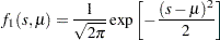
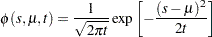
The SEQ call computes, with $\text{[math]}$ , the densities

$\text{[math]}$

with

$\text{[math]}$

and

$\text{[math]}$

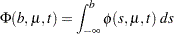
with the associated probability at any point $\text{[math]}$ at level $\text{[math]}$ to be

$\text{[math]}$

with

$\text{[math]}$

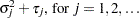
The notation $\text{[math]}$ denotes the vector of time intervals $\text{[math]}$ , and $\text{[math]}$ denotes the probability of continuation at the $\text{[math]}$ th level for a given domain $\text{[math]}$ , a given mean $\text{[math]}$ , and a given time vector $\text{[math]}$ . The variance at the $\text{[math]}$ level can be computed from $\text{[math]}$ .

	$\text{[math]}$	$\text{[math]}$	$\text{[math]}$
	$\text{[math]}$	$\text{[math]}$	$\text{[math]}$

It is important to understand the limitations that are imposed internally on the domain by the numerical method. Any element $\text{[math]}$ will always be limited within a symmetric interval with standardized values not to exceed $\text{[math]}$ . That is,

$\text{[math]}$

SEQSCALE Call

Given a domain $\text{[math]}$ , an optional time vector $\text{[math]}$ , and a probability level $\text{[math]}$ , the SEQSCALE subroutine finds the amount of scaling $\text{[math]}$ that would solve the problem

$\text{[math]}$

The result for the amount of scaling $\text{[math]}$ is returned as the second argument of the SEQSCALE subroutine, scale. Note that because of the complexity of the problem, the SEQSCALE subroutine will not attempt to scale a domain with multiple intervals of continuation.

For a significance level of $\text{[math]}$ , set $\text{[math]}$ .

SEQSHIFT Call

Given a geometry $\text{[math]}$ , an optional time vector $\text{[math]}$ , and a power level $\text{[math]}$ , the SEQSHIFT subroutine finds the mean $\text{[math]}$ that solves $\text{[math]}$ .

Actually, a simple transformation of the variables in the sequential problem yields the following result:

$\text{[math]}$

where $\text{[math]}$ is given by $\text{[math]}$ .

Many options are available with the NLP family of optimization routines, which are described in Chapter 4, "Nonlinear Optimization Subroutines."

Consider the following continuation intervals:

$\text{[math]}$	$\text{[math]}$	$\text{[math]}$
$\text{[math]}$	$\text{[math]}$	$\text{[math]}$
$\text{[math]}$	$\text{[math]}$	$\text{[math]}$
$\text{[math]}$	$\text{[math]}$	$\text{[math]}$

The following statements computes the probability from the sequential test at each boundary point specified in the geometry.

   /* function to insert in m the geometry column a at level k*/
   start table(m,a,k);
      if ncol(m) = 0 & nrow(m) = 0  then    m = j(nrow(a),k,.);
      if nrow(m) < nrow(a) then  m = m// j(nrow(a)-nrow(m),ncol(m),.);
      if ncol(m) < k  then  m = m || j(nrow(m),k-ncol(m),.);
      m[1:nrow(a),k] = a;
   finish;

   call table(m,{-6,2},1);
   call table(m,{-6,3},2);
   call table(m,{-6,4,5,6},3);
   call table(m,{-6,4},4);
   call seq(prob,m) eps = 1.e-8 den="density";
   print m;
   print prob;
   print density;

The following output displays the values returned for $\text{[math]}$ , prob and den, respectively.

The probability at the level $\text{[math]}$ at the point $\text{[math]}$ is prob $\text{[math]}$ , while the density at the same point is density $\text{[math]}$ .

Consider the continuation intervals

$\text{[math]}$	$\text{[math]}$	$\text{[math]}$
$\text{[math]}$	$\text{[math]}$	$\text{[math]}$
$\text{[math]}$	$\text{[math]}$	$\text{[math]}$

Note that the continuation at level 2 can be effectively considered infinite, and it does not numerically affect the results of the computation at level 3. The following statements verify this by using the tscale parameter to compute this problem.

   reset nocenter;
   /* function to insert in m the geometry column a at level k*/
   start table(m,a,k);
      if ncol(m) = 0 & nrow(m) = 0  then    m = j(nrow(a),k,.);
      if nrow(m) < nrow(a) then  m = m// j(nrow(a)-nrow(m),ncol(m),.);
      if ncol(m) < k  then  m = m || j(nrow(m),k-ncol(m),.);
      m[1:nrow(a),k] = a;
   finish;

   call table(m,{-20,2},1);
   call table(m,{-20,20},2);
   call table(m,{-3,3},3);

   /**************************************/
   /* TSCALE has the default value of 1  */
   /**************************************/
   call seq(prob1,m) eps = 1.e-8 den="density";
   print m[format=f5.]  prob1[format=e12.5];

   call table(mm,{-20,2},1);
   call table(mm,{-3,3},2);
      /* You can show a 2-step separation between the levels */
      /* while dropping the intermediate level at 2          */
   tscale = { 2 };
   call seq(prob2,mm) eps = 1.e-8 den="density" TSCALE=tscale;
   print mm[format=f5.]  prob2[format=e12.5];

The output shows the values returned for the variables m, prob1, mm and prob2.

Some internal limitations are imposed on the geometry. Consider the three-level case with geometry $\text{[math]}$ in the preceding statements. Since the tscale variable is not specified, it is set to its default value, $\text{[math]}$ . The variance at the $\text{[math]}$ th level is $\text{[math]}$ for $\text{[math]}$ . The first level has a lower boundary point of $\text{[math]}$ , as represented by the value of $\text{[math]}$ . Since the absolute standardized value is larger than 8, this point is replaced internally by the value $\text{[math]}$ . Hence, the densities and the probabilities reported for the first level at this point are not for the given value $\text{[math]}$ ; instead, they are for the internal value of $\text{[math]}$ . For practical purposes, this limitation is not severe since the absolute error introduced is of the order of $\text{[math]}$ .

The computations performed by the first call of the SEQ subroutine can be simplified since the second level is large enough to be considered infinite. The matrix MM contains the first and third columns of the matrix M. However, in order to specify the two-step separation between the levels, you must specify tscale=2.

This example verifies some of the results published in Table 3 of Pocock (1982). That is, the following statements verify for the given domain that the significance level is $\text{[math]}$ and that the power is $\text{[math]}$ under the alternative hypothesis:

    /*****************************************/
    /* first check whether the numbers yield */
    /* 0.95 for the alpha level              */
    /*****************************************/

    bm      ={-3.663  -2.884 -2.573 -2.375 -2.037,
              -2.988  -2.537 -2.407 -2.346 -2.156,
              -2.598  -2.390 -2.390 -2.390 -2.310,
              -2.446  -2.404 -2.404 -2.404 -2.396};

    bplevel = { 0.5 0.25 0.1  0.05};
    level   = 0.95; /* this the required alpha value  */
    sigma   = diag(sqrt(1:5)); /* global sigma matrix */

    do i = 1 to 4;
       m      = bm[i,];
       plevel = bplevel[i];
       geom   = (m//(-m))*sigma;

       /***************************/
       /* Try the null hypothesis */
       /***************************/

       call seq(prob,geom) eps = 1.e-10;
       palpha  = (prob[2,]-prob[1,])[5];

       /**********************************/
       /* Try the alternative hypothesis */
       /**********************************/

       call seqshift(prob,mean,geom,plevel);
       beta  = (prob[2,] -prob[1,])[5];
       p     = prob[3,]-prob[2,]+prob[1,];

       /**********************************/
       /* Number of patients per group   */
       /**********************************/

       tn    = 4*mean##2;
       maxn  = 5*tn;

       /*************************************/
       /* compute the average sample number */
       /*************************************/

       asn   = tn *( 5 - (4:0) * p`);
       summary = summary // ( palpha  || level || beta ||
                 plevel || tn  || maxn ||asn);
    end;
    print summary[format=10.5];

Note that the variables eps and tscale have been internally set to their default values. The following values are returned for the matrix SUMMARY:

These values compare well with the values shown in Table 3 of Pocock (1982). Differences are of the order of $\text{[math]}$ .

This example shows how to verify the results in Table 1 of Wang and Tsiatis (1987). For a given $\text{[math]}$ , the following program finds $\text{[math]}$ that yields a symmetric continuation interval given by

$\text{[math]}$

with a given significance level of $\text{[math]}$ :

   start func(delta,k) global(level);
      m       = ((1:k))##delta;
      mm      = (-m//m);
      /*******************************/
      /* meet the significance level */
      /* by scaling                  */
      /*******************************/
      call seqscale(prob,scale,mm,level);
      return(scale);
   finish;

   /*********************************/
   /* alpha levels of 0.05 and 0.01 */
   /*********************************/

   blevel        = {0.95 0.99};
   do i = 1 to 2;
      level      = blevel[i];
      free summary;
      do delta   = 0 to .7 by .1;
         free row;
         do k=2 to 5;
            x    = func(delta,k);
            row  = row || x;
         end;
         summary = summary //row;
      end;
      print summary[format=10.5];
   end;

The value of SUMMARY for the 0.95 level is as follows.

The value for SUMMARY for the 0.99 level is as follows.

Note that since eps and tscale are not specified, they are internally set to their default values.

This example verifies the results in Table 2 of Pocock (1977). The following program finds $\text{[math]}$ that yields a symmetric continuation interval given by

$\text{[math]}$

for five groups. The overall significance level is $\text{[math]}$ (the probability $\text{[math]}$ ), and the power is $\text{[math]}$ .

   %let nl = 5;
   start func(plevel) global(level,scale,mean,palpha,beta,tn,asn);
      m       = sqrt((1: &nl));
      mm      =  -m //m;
      /*******************************/
      /* meet the significance level */
      /* by scaling                  */
      /*******************************/

      call seqscale(prob,scale,mm,level);
      palpha  = (prob[2,]-prob[1,])[&nl];
      mm      = mm *scale;

      /*******************************/
      /* meet the power condition    */
      /*******************************/

      call seqshift(prob,mean,mm,plevel);
      return(mean);
   finish;

   /****************/
   /* alpha = 0.95 */
   /****************/

   level   = 9.50000E-01;
   bplevel = { 0.5 .25 .1 0.05 0.01};
   free summary;
   do i = 1 to 5;
      summary = summary || func(bplevel[i]);
   end;
   print summary[format=10.5];

The value returned for SUMMARY are shown in the following table, and the entries agree with Table 2 of Pocock (1977).

            SUMMARY

   0.99359    1.31083    1.59229    1.75953    2.07153

This example illustrates how to find the optimal boundary of the $\text{[math]}$ -class of Wang and Tsiatis (1987). The $\text{[math]}$ -class boundary has the form

$\text{[math]}$

The $\text{[math]}$ -class boundary is optimal if it minimizes the average sample number while satisfying the required significance level $\text{[math]}$ and the required power $\text{[math]}$ . You can use the following program to verify some of the results published in Tables 2 and 3 of Wang and Tsiatis (1987):

   %let nl=5;
   start func(delta) global(level,plevel,mean,
                            scale,alpha,beta,tn,asn);

      m       = ((1: &nl))##delta;
      mm      = (-m//m);

      /*******************************/
      /* meet the significance level */
      /*******************************/

      call seqscale(prob,scale,mm,level);
      alpha   = (prob[2,]-prob[1,])[&nl];
      mm      = mm *scale;

      /*******************************/
      /* meet the power condition    */
      /*******************************/

      call seqshift(prob,mean,mm,plevel);
      beta    = (prob[2,]-prob[1,])[&nl];

      /*************************************/
      /* compute the average sample number */
      /*************************************/

      p       = prob[3,]-prob[2,]+prob[1];
      tn      = 4*mean##2; /* number per group */
      asn     = tn *( &nl - p *(%eval(&nl-1):0)`);
      return(asn);
   finish;

   /**********************************************/
   /* set up the global variables needed by func */
   /**********************************************/

   level   = 0.95;
   plevel  = 0.01;

   /*****************************************/
   /* set up the controlling options of the */
   /* optimization routine                  */
   /*****************************************/

   opt     = {0 2 0 1 6};
   tc      = repeat(.,1,12);
   tc[1]   = 100;
   tc[7]   = 1.e-4;
   par     = { 1.e-13 . 1.e-10 . . .} || . || epsd;

   /*****************************/
   /* provide the initial guess */
   /* and let nlpdd do the work */
   /*****************************/

   delta   = 0.5;
   call nlpdd(rc,rx,"func",delta) opt=opt tc=tc par=par;

The following output displays the results.

                        Optimization Start
                       Parameter Estimates
                                               Gradient
                                              Objective
           N Parameter         Estimate        Function

           1 X1               -1.500000        -8.09752

              Value of Objective Function = 35.232023082

              Double Dogleg Optimization
   Dual Broyden - Fletcher - Goldfarb - Shanno Update (DBFGS)
              Without Parameter Scaling
            Gradient Computed by Finite Differences
          Number of Parameter Estimates 1

            Parameter Estimates                    2
            Functions (Observations)               2

                       Optimization Start

   Active Constraints               0  Criterion = 35.232
   Max Abs Gradient Element     8.098  Radius = 1.000

                   Function    Active      Objective
 Iter    Restart    Calls    Constraints    Function

    1       0          3         0          34.8914
    2*      0          4         0          34.8774
    3*      0          5         0          34.8774

 Iter    difcrit      maxgrad     lambda       slope

    1      0.3406         1.644    49.273     -0.830
    2*     0.0140        0.0440         0    -0.0144
    3*    0.00001       0.00013         0      -1E-5

                  Optimization Results

Iterations                  3  Function Calls              6
Gradient Calls              5  Active Constraints          0
Criterion           34.877417  Max Grad Element  0.000126832
Slope           -0.0000100034  Radius                      1

   NOTE:   FCONV convergence criterion satisfied.

             Optimization Results
             Parameter Estimates

        N Parameter      Estimate      Gradient

        1 X1             0.586554     -0.0001268

       Value of Objective Function = 34.877416815

The optimal function value of 34.88 agrees with the entry in Table 2 of Wang and Tsiatis (1987) for five groups, $\text{[math]}$ , and $\text{[math]}$ . Note that the variables eps and tscale are internally set to their default values. For more information about the NLPDD subroutine, see the section NLPDD Call. For details about the opt, tc, and par arguments in the NLPDD call, see the section Options Vector, the section Termination Criteria, and the section Control Parameters Vector, respectively.

You can replicate other values in Table 2 of Wang and Tsiatis (1987) by changing the values of the variables NL and PLEVEL. You can obtain values from Table 3 by changing the value of the variable LEVEL to 0.99 and specifying NL and PLEVEL accordingly.

This example illustrates how to find the boundaries that minimize ASN given the required significance level and the required power. It replicates some of the results published in Table 3 of Pocock (1982). The program computes the domain that

minimizes the ASN
yields a given significance level of $\text{[math]}$
yields a given power $\text{[math]}$ under the alternative hypothesis

The last two nonlinear conditions on the optimization process can be incorporated as a penalty applied on the error in these nonlinear conditions. The following program does the computations for a power of 0.9.

   %let nl=5;
   start func(m) global(level,plevel,sigma,epss,
                  geometry,stgeom,gscale,mean,alpha,beta,tn,asn);
      m       =  abs(m);
      mm      = ( -m  // m)*sigma;
      /*******************************/
      /* meet the significance level */
      /*******************************/

      call seqscale(prob,gscale,mm,level) iguess=gscale eps=epss;
      stgeom  = gscale*m;
      geometry= mm*gscale;

      alpha   = (prob[2,]-prob[1,])[&nl];

      /*******************************/
      /* meet the power condition    */
      /*******************************/

      call seqshift(prob,mean,geometry,plevel) iguess=mean eps=epss;
      beta    = (prob[2,]-prob[1,])[&nl];
      p       = prob[3,] - prob[2,]+prob[1,];

      /*************************************/
      /* compute the average sample number */
      /*************************************/

      tn      = 4*mean##2; /* number per group */
      asn     = tn *( &nl - p *(%eval(&nl-1):0)`);
      return(asn);
   finish;

   /**********************************************/
   /* set up the global variables needed by func */
   /**********************************************/
   epss    = 1.e-8;
   epso    = 1.e-5;
   level   = 9.50000E-01;
   plevel  = 0.05;
   sigma   = diag(sqrt(1:5));

   /*****************************************/
   /* set up the controlling options of the */
   /* optimization routine                  */
   /*****************************************/

   opt     = {0 2 0 1 6};
   tc      = repeat(.,1,12);
   tc[1]   = 100;
   tc[7]   = 1.e-4;
   par     = { 1.e-13 . 1.e-10 . . .} || . || epso;

   /*************************************/
   /* provide the constraint matrix     */
   /* you need monotonically increasing */
   /* significance levels               */
   /*************************************/

   con     = { .  .  .  .  .    .  . ,
               .  .  .  .  .    .  . ,
               1 -1  .  .  .    1  0 ,
               .  1 -1  .  .    1  0 ,
               .  .  1 -1  .    1  0 ,
               .  .  .  1 -1    1  0 };

   /*****************************/
   /* provide the initial guess */
   /* and let nlp do the work   */
   /*****************************/

   m       = { 1  1  1  1  1  };
   call nlpdd(rc,rx,"func",m) opt=opt blc = con tc=tc par=par;
   print stgeom;

Note that while eps has been set to eps= $\text{[math]}$ , tscale has been internally set to its default value. You can choose to run the program with and without the specification of the keyword IGUESS to see the effect on the execution time.

Note the following about the optimization process:

Different levels of precision are imposed on different modules. In this example, epss, which is used as the precision for the sequential tests, is 1E $\text{[math]}$ 8. The absolute and relative function criteria for the objective function are set to par[7]=1E $\text{[math]}$ 5 and tc[7]=1E $\text{[math]}$ 4, respectively. Since finite differences are used to compute the first and second derivatives, the sequential test should be more precise than the optimization routine. Otherwise, the finite difference estimation is worthless. Optimally, if the precision of the function evaluation is $\text{[math]}$ , the first- and second-order derivatives should be estimated with perturbations $\text{[math]}$ and $\text{[math]}$ , respectively. For example, if all three precision levels are set to 1E $\text{[math]}$ 5, the optimization process does not work properly.
Line search techniques that do not depend on the computation of the derivative are preferable.
The amount of printed information from the optimization routines is controlled by opt[2] and can be set to any value between 0 and 3. Larger numbers produce more output.

Top of Page