The NLPQUA subroutine computes an optimum value of a quadratic objective function.

See the section Nonlinear Optimization and Related Subroutines for a listing of all NLP subroutines. See Chapter 14 for a description of the arguments of NLP subroutines.

The NLPQUA subroutine uses a fast algorithm for maximizing or minimizing the quadratic objective function

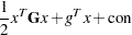subject to boundary constraints and general linear equality and inequality constraints. The algorithm is memory-consuming for problems with general linear constraints.

The matrix must be symmetric but not necessarily positive definite (or negative definite for maximization problems). The constant term affects only the value of the objective function, not its derivatives or the optimal point .

The algorithm is an active-set method in which the update of active boundary and linear constraints is done separately. The decomposition of the matrix of active linear constraints is updated iteratively (see Gill et al. (1984)). If is the number of free parameters (that is, minus the number of active boundary constraints), and is the number of active linear constraints, then is an orthogonal matrix that contains null space in its first columns and range space in its last columns. The matrix is an triangular matrix of the form for . The Cholesky factor of the projected Hessian matrix is updated simultaneously with the decomposition when the active set changes.

The objective function is specified by the input arguments quad and lin, as follows:

• The quad argument specifies the symmetric Hessian matrix, , of the quadratic term. The input can be in dense or sparse form. In dense form, all entries of the quad matrix must be specified. If , the dense specification must be used. The sparse specification can be useful when has many zero elements. You can specify an matrix in which each row represents one of the nonzero elements of . The first column specifies the row location in , the second column specifies the column location, and the third column specifies the value of the nonzero element.

• The lin argument specifies the linear part of the quadratic optimization problem. It must be a vector of length or . If lin is a vector of length , it specifies the vector of the linear term, and the constant term is considered zero. If lin is a vector of length , then the first elements of the argument specify the vector and the last element specifies the constant term of the objective function.

As in the other optimization subroutines, you can use the blc argument to specify boundary and general linear constraints, and you must provide a starting point x0 to determine the number of parameters. If x0 is not feasible, a feasible initial point is computed by linear programming, and the elements of x0 can be missing values.

Assuming nonnegativity constraints , the quadratic optimization problem solved with the LCP call, which solves the linear complementarity problem.

Choosing a sparse (or dense) input form of the quad argument does not mean that the algorithm used in the NLPQUA subroutine is necessarily sparse (or dense). If the following conditions are satisfied, the NLPQUA algorithm will store and process the matrix as sparse:

• No general linear constraints are specified.

• The memory needed for the sparse storage of is less than 80% of the memory needed for dense storage.

• is not a diagonal matrix. If is diagonal, it is stored and processed as a diagonal matrix.

The sparse NLPQUA algorithm uses a modified form of minimum degree Cholesky factorization (George and Liu; 1981).

In addition to the standard iteration history, the NLPNRA subroutine prints the following information:

• The heading alpha is the step size, , computed with the line-search algorithm.

• The heading slope refers to , the slope of the search direction at the current parameter iterate . For minimization, this value should be significantly smaller than zero. Otherwise, the line-search algorithm has difficulty reducing the function value sufficiently.

The Betts problem (see the section Constrained Betts Function) can be expressed as a quadratic problem in the following way:

Then

The following statements use the NLPQUA subroutine to solve the Betts problem:

   lin  = { 0. 0. -100};
   quad = {  0.02   0.0 ,
             0.0    2.0 };
   c    = {  2. -50.  .   .,
            50.  50.  .   .,
            10.  -1. 1. 10.};
   x = { -1. -1.};
   optn = {0 2};
   CALL NLPQUA(rc,xres,quad,x,optn,c,,,,lin);

The quad argument specifies the matrix, and the lin argument specifies the vector with the value of con appended as the last element. The matrix c specifies the boundary constraints and the general linear constraint.

The iteration history follows.

                         Optimization Start
                         Parameter Estimates
                                      Gradient           Lower           Upper
                                      Objective           Bound           Bound
  N Parameter         Estimate        Function      Constraint      Constraint

  1 X1                6.800000        0.136000        2.000000       50.000000
  2 X2               -1.000000       -2.000000      -50.000000       50.000000

          Value of Objective Function = -98.5376

                      Linear Constraints

  1   59.00000 :  10.0000 <= + 10.0000 * X1 - 1.0000 * X2

                 Null Space Method of Quadratic Problem

                  Parameter Estimates                2
                  Lower Bounds                       2
                  Upper Bounds                       2
                  Linear Constraints                 1
                  Using Sparse Hessian               _

                   Optimization Start

   Active Constraints        0  Objective Function  -98.5376
   Max Abs Gradient Element  2

                    Function        Active       Objective
 Iter    Restarts      Calls   Constraints        Function

    1           0          2             1       -99.87349
    2           0          3             1       -99.96000

        Objective    Max Abs              Slope of
         Function   Gradient      Step      Search
 Iter      Change    Element      Size   Direction

    1      1.3359     0.5882     0.706      -2.925
    2      0.0865          0     1.000      -0.173

                            Optimization Results

Iterations                             2  Function Calls            4
Gradient Calls                         3  Active Constraints        1
Objective Function                -99.96  Max Abs Gradient Element  0
Slope of Search Direction   -0.173010381

   ABSGCONV convergence criterion satisfied.

                     Optimization Results
                     Parameter Estimates

                                      Gradient    Active
                                      Objective    Bound
  N Parameter         Estimate        Function    Constraint

  1 X1                2.000000        0.040000     Lower BC
  2 X2                       0               0

             Value of Objective Function = -99.96

         Linear Constraints Evaluated at Solution

 1    10.00000 = -10.0000 + 10.0000 * X1 - 1.0000 * X2