The ITSOLVER subroutine solves a sparse linear system by using iterative methods.

The ITSOLVER call returns the following values:

x

is the solution to .

error

is the final relative error of the solution.

iter

is the number of iterations executed.

The input arguments to the ITSOLVER call are as follows:

method

is the type of iterative method to use.

A

is the sparse coefficient matrix in the equation . You can use SPARSE function to convert a matrix from dense to sparse storage.

b

is a column vector, the right side of the equation .

precon

is the name of a preconditioning technique to use.

tol

is the relative error tolerance.

maxiter

is the iteration limit.

start

is a starting point column vector.

history

is a matrix to store the relative error at each iteration.

The ITSOLVER call solves a sparse linear system by iterative methods, which involve updating a trial solution over successive iterations to minimize the error. The ITSOLVER call uses the technique specified in the method parameter to update the solution. The valid method options are as follows:

method = "CG":

conjugate gradient algorithm, when A is symmetric and positive definite.

method = "CGS":

conjugate gradient squared algorithm, for general A.

method = "MINRES":

minimum residual algorithm, when A is symmetric indefinite.

method = "BICG":

biconjugate gradient algorithm, for general A.

The input matrix represents the coefficient matrix in sparse format; it is an 3 matrix, where is the number of nonzero elements. The first column contains the nonzero values, while the second and third columns contain the row and column locations for the nonzero elements, respectively. For the algorithms assuming symmetric , conjugate gradient, and minimum residual, only the lower triangular elements should be specified. The algorithm continues iterating to improve the solution until either the relative error tolerance specified in is satisfied or the maximum number of iterations specified in is reached. The relative error is defined as

where the operator is the Euclidean norm, and is a machine-dependent epsilon value to prevent any division by zero. If or is not specified in the call, then a default value of is used for and 100000 for .

The convergence of an iterative algorithm can often be enhanced by preconditioning the input coefficient matrix. The preconditioning option is specified with the parameter, which can take one of the following values:

precon = ’NONE’:

no preconditioning

precon = ’IC’:

incomplete Cholesky factorization, for = ’CG’ or ’MINRES’ only

precon = ’DIAG’:

diagonal Jacobi preconditioner, for = ’CG’ or ’MINRES’ only

precon = ’MILU’:

modified incomplete LU factorization, for = ’BICG’ only

If is not specified, no preconditioning is applied.

A starting trial solution can be specified with the parameter; otherwise the ITSOLVER call generates a zero starting point. You can supply a matrix to store the relative error at each iteration with the parameter. The matrix should be dimensioned with enough elements to store the maximum number of iterations you expect.

You should always check the returned and parameters to verify that the desired relative error tolerance is reached. If not, the program might continue the solution process with another ITSOLVER call, with set to the latest result. You might also try a different option to enhance convergence.

For example, the following linear system has a coefficient matrix that contains several zeroes:

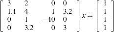You can represent the matrix in sparse form and use the biconjugate gradient algorithm to solve the linear system, as shown in the following statements:

/* value     row column */
A = {  3       1      1,
       2       1      2,
       1.1     2      1,
       4       2      2,
       1       3      2,
       3.2     4      2,
     -10       3      3,
       3       4      4};

/* right hand side */
b = {1, 1, 1, 1};
maxiter = 10;
hist = j(maxiter,1,.);
start = {1,1,1,1};
tol = 1e-10;
call itsolver(x, error, iter, "bicg", A, b, "milu", tol, 
maxiter, start, hist);
print x;
print iter error;
print hist;

The following linear system also has a coefficient matrix with several zeroes:

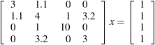The following statements represent the matrix in sparse form and use the conjugate gradient algorithm solve the symmetric positive definite system:

/* value     row column */
A = { 3       1      1,
      1.1     2      1,
      4       2      2,
      1       3      2,
      3.2     4      2,
     10       3      3,
      3       4      4};

/* right hand side */
b = {1, 1, 1, 1};
call itsolver(x, error, iter, "CG", A, b);
print x, iter, error;