Data Smoothing: Loess

Example: Compare Smoothers

Subsections:

Removing a Smoother

The "Details" section of the LOESS procedure documentation describes how the LOESS procedure computes predicted values. The predicted value at a point x is determined by a weighted average of observations near x. The number of observations used to form the predicted value depends on the smoothing parameter.

Recall that the response variable in the previous example is the length of time required to drill the last five feet of a hole that is depth feet deep. For these data, the optimal smoothing parameter was approximately 0.131. This value results in a smoother that varies with the hardness of the underlying rock strata.

However, you might want to average out the variations in rock hardness to get a better indication of how the drilling time varies with depth. While 0.131 is a global minimum of the AICC function, there might be a local minimum at a larger value of the smoothing parameter. Using a larger value results in a smoother that is less sensitive to local variation in rock hardness.

This example computes another possible loess fit and compares it to the smoother with the parameter 0.131. The example assumes you have completed the previous example and your workspace looks like Figure 18.5.

Recall that SAS/IML Studio adds a smoother to an existing scatter plot when both of the following conditions are satisfied:

The scatter plot is the active window when you select the analysis.
The scatter plot variables match the analysis variables.

To compute a second loess fit and compare the two models:

Click the scatter plot of driltime versus depth to activate that window.
Select Analysis →Data Smoothing →Loess from the main menu.

The loess dialog box appears. The dialog box remembers the variables you used in the last analysis.
Make sure that driltime is selected as the Y variable and depth is selected as the X variable.

By examining the AICC plot from the previous example (upper left in Figure 18.5), you might guess that the AICC is an increasing function of the smoothing parameter on the interval $[0.131, 0.5]$ . Thus, if there is a local minimum for AICC at a larger value of the smoothing parameter, it must occur in the interval $[0.5, 1]$ . In the following steps you search for a local minimum of AICC restricted to this interval.
Click the Method tab.

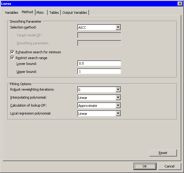
The Method tab is activated, as shown in Figure 18.6.

Figure 18.6: The Method Tab
Click Exhaustive search for minimum.
Click Restrict search range and type 0.5 for the Lower bound.

Note: The Exhaustive search for minimum option is computationally expensive. It corresponds to the GLOBAL modifier of the SELECT= option in the LOESS MODEL statement. For the current example, which has 80 observations, the option results in evaluating loess models with at least 40 ( $0.5 \times 80$ ) points in the local neighborhoods. Thus, this option causes the LOESS procedure to evaluate many separate models: one with 40 points in the local neighborhoods, one with 41 points, and so on, up to 80 points. For a data set with 10,000 observations, the same options would result in evaluating up to 5,000 models.
Click the Plots tab.

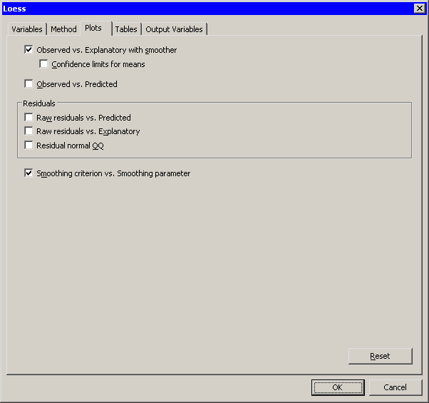
The Plots tab is activated, as shown in Figure 18.7.

Figure 18.7: Selecting Plots
Clear Raw residuals vs. Explanatory.
Click OK.

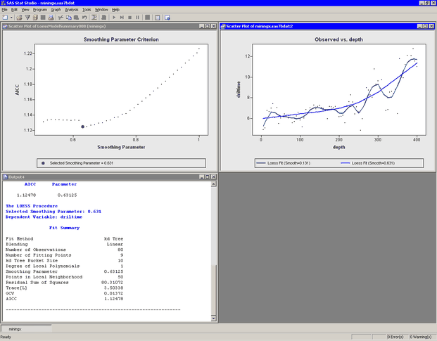
As shown in Figure 18.8, the scatter plot of driltime versus depth updates to display the new loess smoother. The AICC plot now shows that the chosen smoothing parameter is approximately 0.631, which corresponds to using 50 ( $\approx 0.631 \times 80$ ) points in the local neighborhoods.

Figure 18.8: Example: Rerun a Loess Analysis

Note: This second Loess analysis creates a predicted value variable named LoessP_driltime. This variable overwrites the variable of the same name that was created by the first Loess analysis. If you want to compare the predicted values for these two models, you need to rename the first variable prior to running the second analysis.