Distribution Analysis: Distributional Modeling
In this example, you fit a normal distribution to the pressure_outer_isobar variable of the Hurricanes data set. The Hurricanes data set contains 6,188 observations of tropical cyclones in the Atlantic basin. The pressure_outer_isobar variable gives the sea-level atmospheric pressure for the outermost closed isobar of a cyclone. This is a measure of the
atmospheric pressure at the outermost edge of the storm.
The plots and statistics in the Distributional Modeling analysis can help you answer questions such as the following:
-
Can these data be modeled by a parametric distribution? For example, are the data normally distributed?
-
If not, which characteristics of the data depart from the fitted distribution? For example, is the data distribution long-tailed? Is it skewed?
-
What proportion of the data is within a given range of values?
Answers to these questions for the pressure_outer_isobar variable appear at the end of this example.
-
Open the
Hurricanesdata set. -
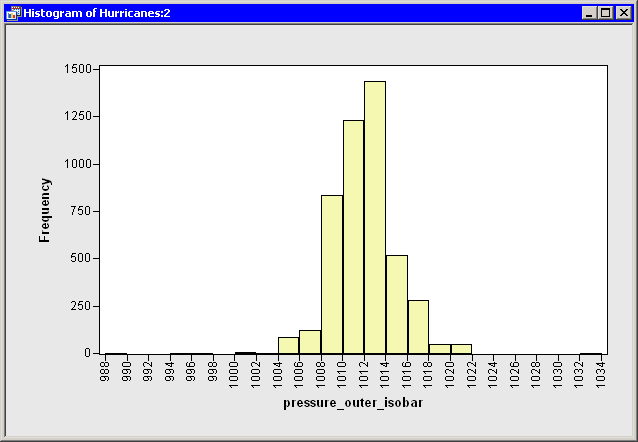
Create a histogram of the
pressure_outer_isobarvariable.A histogram appears, as shown in Figure 15.1.
From the shape of the histogram you might wonder if the data distribution can be modeled by a normal distribution. If not, how do these data deviate from normality? The following steps add a normal curve to the histogram and create other plots and statistics.
-
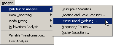
Select → → from the main menu, as shown in Figure 15.2.
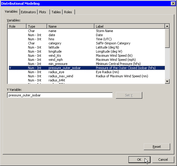
The Distrbutional Modeling dialog box appears. (See Figure 15.3.) You can select a variable for the univariate analysis by using the Variables tab.
-
Select the variable
pressure_outer_isobar, and click . -
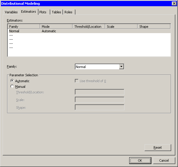
Click the Estimators tab.
The Estimators tab is shown in Figure 15.4.
The Estimators tab enables you to select distributions to fit to the data. For each distribution, you can enter known parameters or indicate that the parameters should be estimated by maximum likelihood.
The section Example: Specify Multiple Density Curves describes how to create a histogram overlaid with more than one density curve. For this example, you select a single distribution to fit to the data.
The normal distribution appears in the list by default. Also by default, the radio button is selected. This specifies that the location and scale parameters for the normal distribution be determined by using maximum likelihood estimation.
Accept these defaults and proceed to the next tab.
-
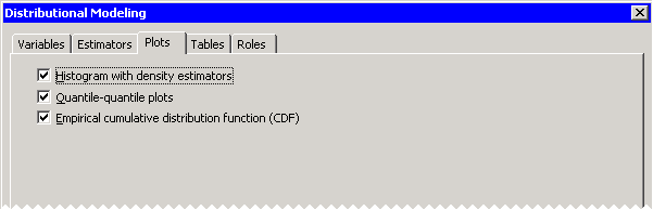
Click the Plots tab.
-
Select all plots, as shown in Figure 15.5.
-
Click .
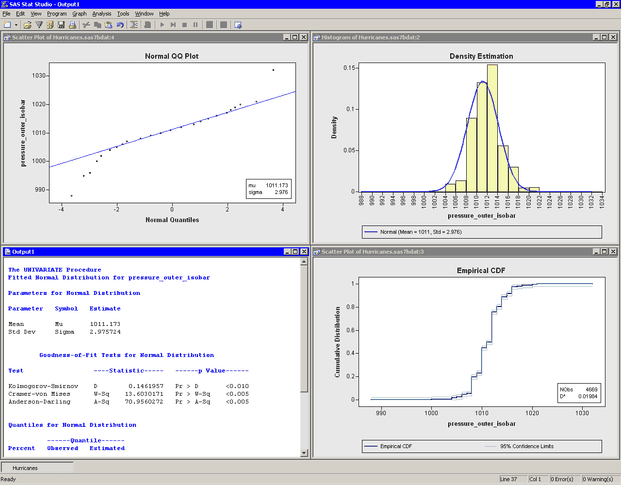
The analysis calls the UNIVARIATE procedure, which uses the options specified in the dialog box. The procedure displays tables in the output document, as shown in Figure 15.6.
Several plots are created. These plots can help answer the questions posed earlier.