Transformations for Proportion Variables :: SAS/IML(R) Studio 13.1: User's Guide

Transformations for Proportion Variables

Subsections:

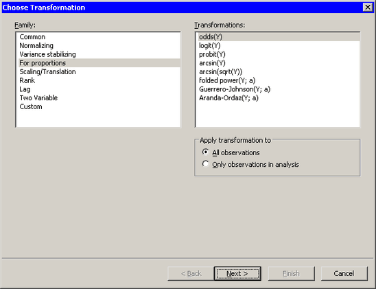
Figure 32.14 shows the transformations that are available when you select For proportions from the Family list. These transformations are intended for variables that represent proportions. That is, the $Y$ variable must take values between 0 and 1. You can also use these transformations for percentages if you first divide the percentages by 100.

Chapter 7 of Atkinson (1985) is devoted to transformations of proportions. Equations for these transformations are given in Table 32.4.

Figure 32.14: Transformations for Proportions

Table 32.4: Description of Transformations for Proportions $Y\in [0,1)$

Transformation	Parameter	New Variable	Equation
	Default	Name of
odds(Y)		Odds_Y	$Y/(1-Y)$
logit(Y)		Logit_Y	$\log (Y/(1-Y))$
probit(Y)		Probit_Y	$\mbox{probit}(Y)$
arcsin(Y)		Arcsin_Y	$\arcsin (Y)$
arcsin(sqrt(Y))		Angular_Y	$\arcsin (\sqrt {Y})$
folded power(Y;a)	MLE	FPow_Y	See text.
Guerrero-Johnson(Y;a)	MLE	GJ_Y	See text.
Aranda-Ordaz(Y;a)	MLE	AO_Y	See text.

The probit function is the quantile function of the standard normal distribution.

The last three transformations in the list are similar to the Box-Cox transformation described in the section Normalizing Transformations. The parameter for each transformation is in the unit interval: $a\in [0,1]$ . Typically, you choose a parameter that maximizes (or nearly maximizes) a log-likelihood function.

The log-likelihood function is defined as follows. Let $N$ be the number of nonmissing values, and let $G(\cdot )$ be the geometric mean function. Each transformation has a corresponding normalized transformation $\bm {z}(\lambda ; y)$ , to be defined later. Define

$R(\lambda ;\bm {z}) = \bm {z}’\bm {z} - \left(\Sigma z_ i \right)^2 / N$

and define the log-likelihood function as

$L(\lambda ;\bm {z}) = -(N/2) \log (R(\lambda ;\bm {z})/(N-1))$

The following sections define the normalized transformation for the folded power, Guerrero-Johnson, and Aranda-Ordaz transformations. In each section, $p=y/(1-y)$ .