Example: Fit a Loess Curve to Data :: SAS/IML(R) Studio 13.1: User's Guide

Example: Fit a Loess Curve to Data

In this example, you fit a loess curve to data in the miningx data set. The miningx data set contains 80 observations that correspond to a single test hole in the mining data set. The driltime variable is the time that is required to drill the last five feet of the current depth, in minutes; the current depth is recorded in the depth variable.

To fit a loess curve:

Open the miningx data set.
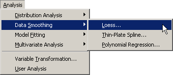
Select Analysis →Data Smoothing →Loess from the main menu, as shown in Figure 18.2.

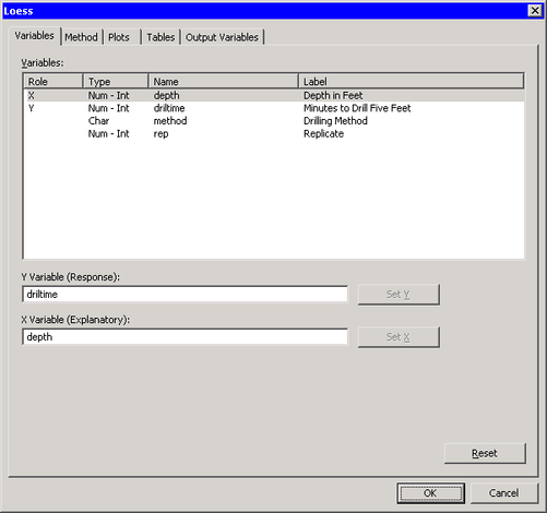
Figure 18.2: Selecting the Loess Analysis

The Loess dialog box appears. You can select variables for the analysis by using the Variables tab, shown in Figure 18.3.
Select the variable driltime, and click Set Y.
Select the variable depth and click Set X.

Figure 18.3: Selecting Variables
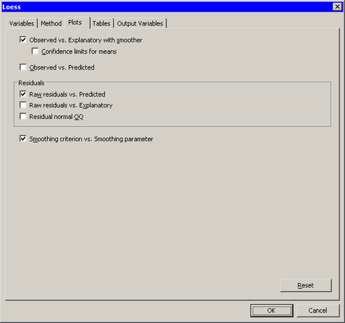
Click the Plots tab.

The Plots tab becomes active. (See Figure 18.4.) You can use this tab to request additional plots.
Select Raw residuals vs. Explanatory.

For this example it is useful to request a plot of the smoothing criterion versus the smoothing parameter. The loess smoothing parameter determines the percentage of observations used to fit a weighted regression in each local neighborhood. Small values of the smoothing parameter often correspond to undersmoothed curves with many undulations; large values correspond to oversmoothed curves with few undulations. The parameter value that minimizes the smoothing criterion represents a compromise between model fit and model complexity.
Select Smoothing criterion vs. Smoothing parameter.
Click OK.

Figure 18.4: Selecting Plots

The Loess analysis calls the LOESS procedure with the options specified in the dialog box. The procedure displays two tables in the output document, as shown in Figure 18.5. The first table shows that the minimum value of the bias-corrected Akaike’s information criterion (AICC) was achieved for a smoothing parameter of $0.13125$ . The second table summarizes the options used by the LOESS procedure and also summarizes the loess fit.

Three plots are created. Some plots might be hidden beneath others. If so, move the plots so that the workspace looks like Figure 18.5.

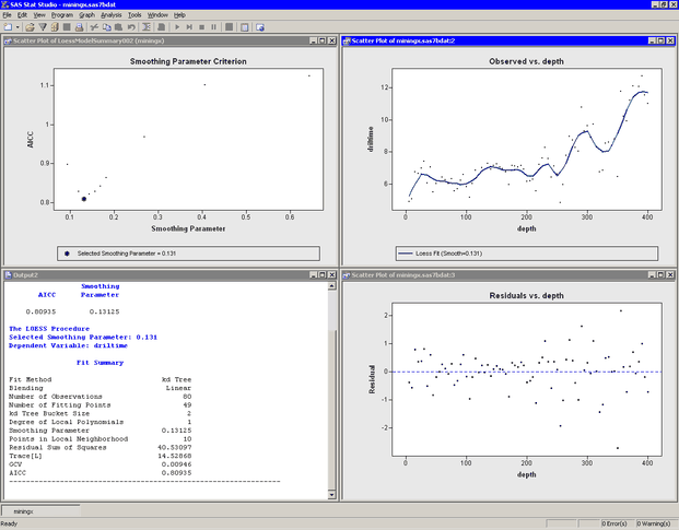
Figure 18.5: Output from a Loess Analysis

One plot (upper left in Figure 18.5) shows the AICC for each value of the smoothing parameter evaluated by the LOESS procedure. Note that the selected smoothing parameter is the one that minimizes the AICC.

A second plot (upper right in Figure 18.5) shows a scatter plot of driltime versus depth, with a loess smoother overlaid. The undulations in the smoother might correspond to depths at which variations in rock hardness affect the drilling time. In particular, it is known that the decrease in drilling time at 250 feet is due to encountering a layer of soft copper-nickel ore (Penner and Watts, 1991).

The third plot (lower right in Figure 18.5) shows the residuals versus depth. The spread of the residuals suggests that the variance of the drilling time is a function of the depth of the hole being drilled.

The next example creates a second curve that smooths out some of the undulations. This is accomplished by restricting the smoothing parameter to relatively large values. Specifically, the next example specifies that at least 50% of the points in the data set should be used for each local weighted regression.