Example: Reduce Dimensionality through Common Factor Analysis

This example investigates factors that explain several variables in the Baseball data set. The Baseball data set contains performance measures for major league baseball players in 1986. A full description of the Baseball data is included in Appendix A: Sample Data Sets.

Suppose you postulate the existence of latent variables that explain the hitting and fielding performance of players’ performances during the 1986 season. (An example of a latent variable in the context of baseball is “quickness,” which could explain correlation between a player’s runs, stolen bases, and fielding statistics.) There are six variables that measure a player’s batting performance: no_atbat, no_hits, no_home, no_runs, no_rbi, and no_bb. There are three variables that measure a player’s fielding performance: no_outs, no_assts, and no_error.

To form a low-dimensional factor space that explains the relationships among these nine variables:

Open the Baseball data set.
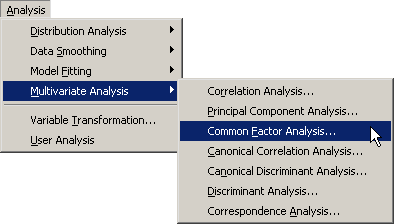
Select Analysis →Multivariate Analysis →Factor Analysis from the main menu, as shown in Figure 27.2.

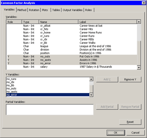
Figure 27.2: Selecting the Factor Analysis

The Factor Analysis dialog box appears. (See Figure 27.3.) You can select variables for the analysis by using the Variables tab.
Select no_atbat. While holding down the CTRL key, select no_hits, no_home, no_runs, no_rbi, and no_bb. Click Add Y.

Note: Alternately, you can select the variables by using contiguous selection: click the first item, hold down the SHIFT key, and click the last item. All items between the first and last item are selected and can be added by clicking Add Y.

The three measures of fielding performance are located near the end of the list of variables.
Scroll to the end of the variable list. Select no_outs. While holding down the CTRL key, select no_assts and no_error. Click Add Y.

Figure 27.3: The Variables Tab
Click the Method tab.

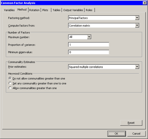
The Method tab becomes active. (See Figure 27.4.) You can use the Method tab to set options in the analysis.

The default method is principal factor analysis. However, the default method of estimating the prior communalities is to set all prior communalities to 1. This would result in a principal component analysis rather than a factor analysis.
Set Prior estimates to Squared multiple correlations.

The preceding step sets the prior communality estimate for each variable to its squared multiple correlation with all other variables.

Figure 27.4: The Method Tab
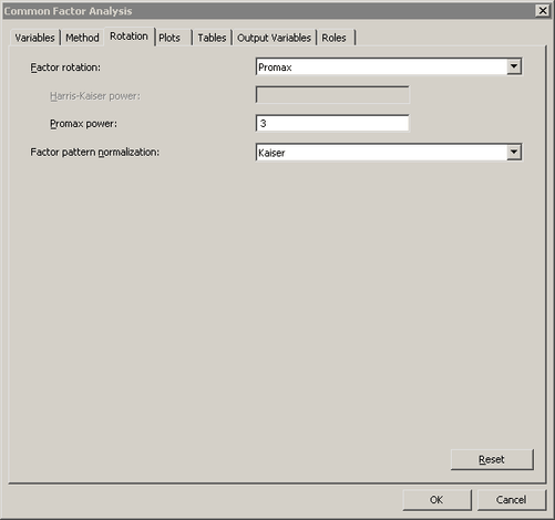
Click the Rotation tab.

The Rotation tab becomes active. (See Figure 27.5.) The default behavior is to leave factors unrotated. This example requests that an oblique transformation be applied to the factors in order to illustrate how rotated factors can sometimes be more interpretable.
Select Promax for the Factor rotation option.

Figure 27.5: The Rotation Tab
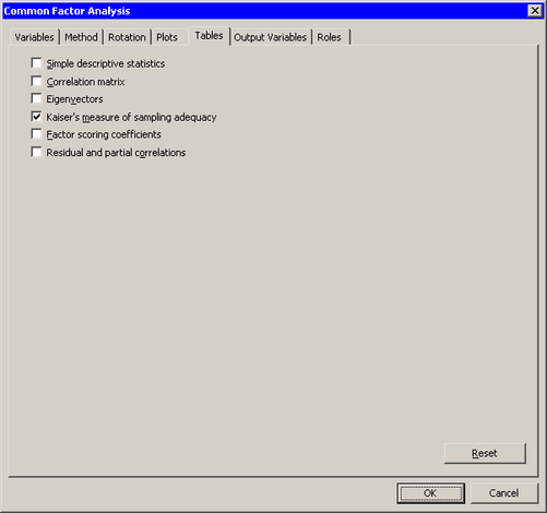
Click the Tables tab.

The Tables tab becomes active. (See Figure 27.6.) To help determine whether the data are appropriate for the common factor model, you can request Kaiser’s measure of sampling adequacy (MSA).
Select Kaiser’s measure of sampling adequacy.
Click OK.

Figure 27.6: The Tables Tab

The analysis calls the FACTOR procedure, which uses the options specified in the dialog box. The procedure displays tables in the output document, as shown in Figure 27.7. As is discussed subsequently, the Factor analysis extracts three principal factors for these data. Three plots also appear.

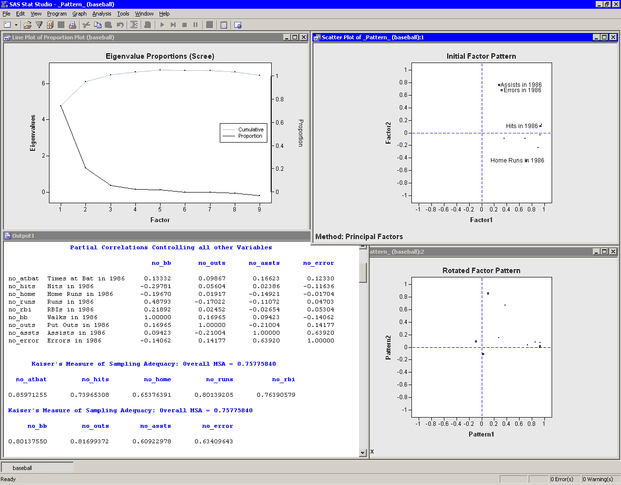
Figure 27.7: Output from a Factor Analysis

The eigenvalue plot shows the eigenvalues of the reduced correlation matrix, along with the cumulative proportion of common variance accounted for by the factors. The first two factors account for almost 95% of the common variance, and the first three factors account for 101%. The reduced correlation matrix for these data has negative eigenvalues, which explains why the factors that correspond to the largest eigenvalues account for more than 100% of the common variance.

The initial factor pattern plot shows the projection of the original variables onto the subspace spanned by the first two factors. As shown in Figure 27.7, you can click a point in order to identify the corresponding variable. The points with high values of Factor1 are all hitting variables, including no_hits. The points with the highest values of Factor2 are two of the fielding variables: no_assts and no_error. The third fielding variable (no_outs) is closest to the origin in this plot. The initial factor pattern plot indicates that the first (unrotated) factor correlates highly with the hitting variables, whereas the second correlates with assists and errors.

Note: If you want to visualize the third extracted factor, you can color the observations according to the value of the Factor3 variable or create a three-dimensional scatter plot of the three factors. You can view the data for this plot by pressing the F9 key when the plot is active.

The rotated factor pattern plot in Figure 27.7 shows the projection of the original variables onto the subspace spanned by the first two rotated factors. A promax transformation is used to transform the original factors (which are orthogonal to each other) to new factors that, in many cases, are easier to interpret in terms of the original variables. This transformation does not change the common factor space or the communality estimates.

In the rotated factor pattern plot, the cluster of points with high values of Pattern1 are the variables no_atbat, no_hits, no_runs, and no_bb. (These points are not labeled in Figure 27.7, but they are labeled in Figure 27.8.) Players with high values of these variables get on base often, so you might interpret the first (rotated) factor to be “Getting on Base.” The two points with high values of Pattern2 are the variables no_home and no_rbi. Players who have high values of these variables contribute many runs to their teams’ scores, so you might interpret the second (rotated) factor as “Scoring.”

In the rotated factor pattern plot, the fielding variables are positioned near the origin, which indicates that these variables are not strongly correlated with the first two rotated factors. Figure 27.8 shows a three-dimensional scatter plot that visualizes the three rotated factors. The plot shows that no_assts and no_error are highly correlated with the third rotated factor, while no_outs is not strongly correlated with any of the first three factors. The third rotated factor identifies players who make many assists and many errors. These are typically infielders who play second base, shortstop, or third base. Consequently, you might interpret the third rotated factor as a “Fielding Position” factor.

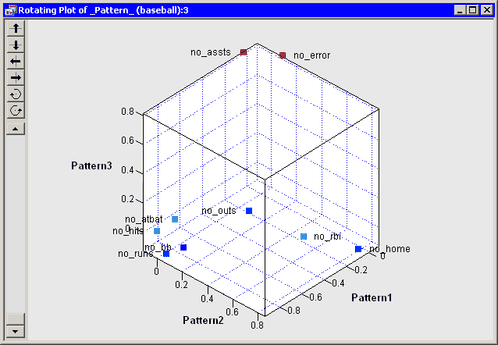
Figure 27.8: Plot of Obliquely Transformed Factors

Figure 27.7 shows part of the partial correlations matrix for the original variables. If the data are appropriate for the common factor model, the partial correlations (controlling the other variables) should be small compared to the original correlations. Recall that the partial correlation between two variables, controlling for the variables $X_1, \ldots , X_ k$ , is the correlation between the residuals of the two variables after regression on the $X_ i$ .

Figure 27.7 also shows the MSA statistics. Kaiser’s MSA (Kaiser, 1970) is a summary, for each variable and for all variables together, of how much smaller the partial correlations are than the original correlations. Values of 0.8 or 0.9 are considered good, while MSAs less than 0.5 are unacceptable. The no_assts and no_error variables have the poorest MSAs. The overall MSA of 0.76 is adequate for proceeding with the factor analysis; an overall MSA lower than 0.6 often indicates that the data are not likely to factor well.

Figure 27.9 shows additional output. The prior communality estimates indicate that the variance of no_outs might not be well explained by the three common factors. The table of eigenvalues displays the eigenvalues for the reduced correlation matrix, which is the correlation matrix of the original variables, except that the 1’s on the diagonal are replaced by the prior communality estimates. A note is printed below this table which indicates that three factors are retained because they account for (at least) 100% of the common variance.

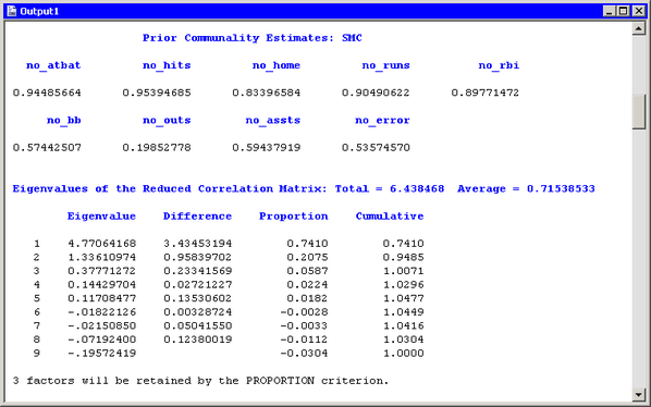
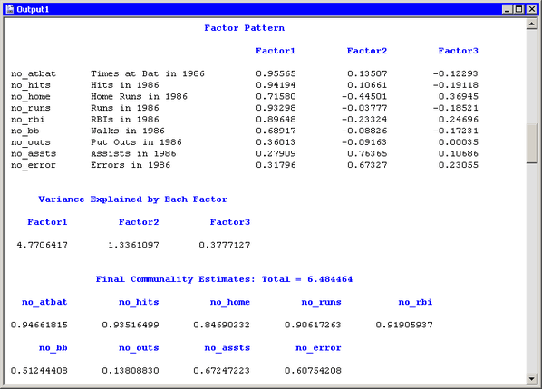
Figure 27.9: Output from a Factor Analysis

Figure 27.10 shows additional output from the FACTOR procedure. The “Factor Pattern” table shows the relationship between the unrotated factors and the original Y variables. Each Y variable is a linear combinations of the common factor and a unique factor. For example, no_atbat corresponds to the linear combination

$\mbox{\Variable{no\_ atbat}} = 0.95565 \: \mbox{\Variable{Factor1}} + 0.13507 \: \mbox{\Variable{Factor2}} - 0.12293 \: \mbox{\Variable{Factor3}} + u_1$

If you decide not to rotate the factors, you can attempt to interpret these factors by looking at the relative magnitudes of the coefficients. For example, the first unrotated factor appears to measure a player’s overall performance. More weight is given to getting on base (coefficients in the range 0.89–0.96), less weight is given to scoring runs (coefficients in the range 0.68–0.72), and little weight is given to the fielding statistics. The figure also shows the common variance explained by each factor and the final communality estimates.

Figure 27.10: Unrotated Factors

Whereas Figure 27.10 displays information about the unrotated factors, Figure 27.11 displays information about the rotated factors. The promax transformation is the composition of two transformations: an orthogonal varimax rotation and an oblique Procrustean transformation. Figure 27.11 displays information about the factors after the orthogonal varimax rotation. You can also visualize the pattern of the rotated factors as follows: view the data for a factor pattern plot by pressing the F9 key when the factor pattern plot is active, and then create scatter plots of the variables named Prerotat $n$ . The Prerotat $n$ variables correspond to the columns of the “Rotated Factor Pattern Table.”

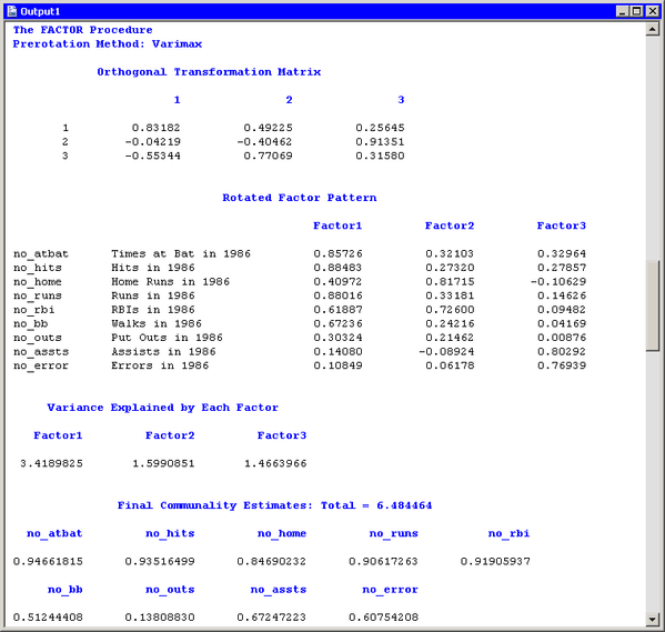
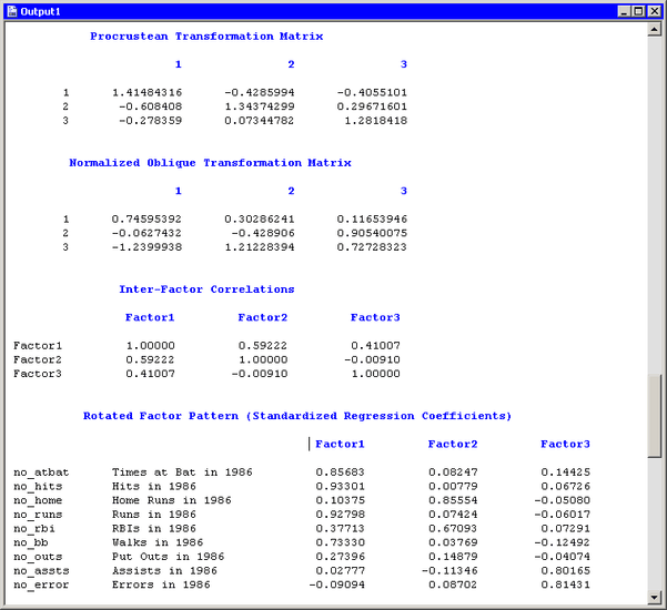
Figure 27.11: Orthogonally Rotated Factors

Figure 27.12 displays information about the obliquely transformed factors. The Procrustean transformation is displayed, followed by the matrix used to transform the unrotated factors into the factors displayed in the “Rotated Factor Pattern (Standardized Regression Coefficients)” table. The factor loadings shown in this table are shown graphically in the rotated factor pattern plot. (See Figure 27.7.) An oblique transformation introduces correlations between the factors, and the “Inter-Factor Correlations” table shows those correlations. You can convert the correlations into angles between the factors by applying the arccosine function. For example, the angle between the first and second factors is $\cos ^{-1}(0.59222)$ , or approximately 53.7 degrees, whereas the second and third factors are almost orthogonal.

The output contains additional tables (not shown) that display further correlations, structures, and variances. The “Displayed Output” section of the FACTOR procedure documentation describes all of the tables.

Figure 27.12: Obliquely Rotated Factors