Example: Analyze the Relationship between Two Groups of Variables

In this example, you examine canonical correlations between sets of variables in the GPA data set. The GPA data set contains average high school grades in mathematics, science, and English for students that applied to a university computer science program. The data also contains the students’ scores on the mathematics and verbal sections of the SAT, which is a standardized test to measure aptitude.

Suppose you are interested in the relationship between the variables that represent analytical thinking and those that represent verbal thinking. You can group the following variables into the analytical set: hsm (high school math average), hss (high school science average), and satm (SAT math score). You can group the following variables into the verbal set: hse (high school English average) and satv (SAT verbal score).

To run a canonical correlation analysis:

Open the GPA data set.
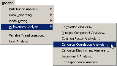
Select Analysis →Multivariate Analysis →Canonical Correlation Analysis from the main menu, as shown in Figure 28.1.

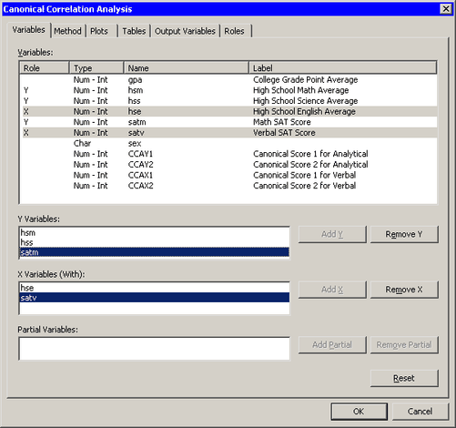
Figure 28.1: Selecting the Canonical Correlation Analysis

The Canonical Correlation Analysis dialog box appears. (See Figure 28.2.) You can select variables for the analysis by using the Variables tab.
Select hsm. While holding down the CTRL key, select hss and satm. Click Add Y.
Select hse. While holding down the CTRL key, select satv. Click Add X.

Figure 28.2: The Variables Tab
Click the Tables tab.

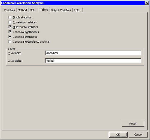
The Tables tab becomes active. (See Figure 28.3.) You can use the Tables tab to display statistics that are associated with the analysis, and to specify labels that identify the two sets of variables.

For this example, you can label the first set of variables as the “Analytical” set and the second set as the “Verbal” set.
Type Analytical into the Y variables field.
Type Verbal into the X variables field.

Figure 28.3: The Tables Tab
Click OK.

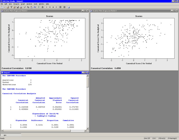
The analysis calls the CANCORR procedure, which uses the options specified in the dialog box. The procedure displays tables in the output document, as shown in Figure 28.4. Two plots are also created.

The plot of the first canonical variables shows the strength of the relationship between the set of analytical variables and the set of verbal variables. The second plot shows the second canonical variables. The footnote of these plots displays the canonical correlations. Note that the correlation between the second pair of canonical variables is less than the correlation between the first pair.

The output window in Figure 28.4 displays the canonical correlation, which is the correlation between the first pair of canonical variables. The value 0.6106 represents the highest possible correlation between any linear combination of the analytical variables and any linear combination of the verbal variables.

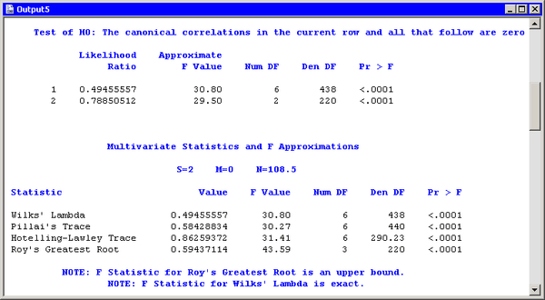
Figure 28.4: Output from a Canonical Correlation Analysis

The output window contains additional tables, as shown in Figure 28.5. The figure displays the likelihood ratios and associated statistics for testing the hypothesis that the canonical correlations in the current row and all that follow are zero. The first approximate $F$ value of 30.80 corresponds to the test that all canonical correlations are zero. Since the $p$ -value is small, you can reject the null hypothesis at the 95% level. Similarly, the second approximate $F$ value of 29.50 corresponds to the test that the second canonical correlation is zero. This test also rejects the hypothesis.

Several multivariate statistics and $F$ test approximations are also provided. These statistics test the null hypothesis that all canonical correlations are zero. The small $p$ -values for these tests (< 0.0001) are evidence for rejecting the null hypothesis.

Figure 28.5: Testing Whether Canonical Correlations Are Zero

The analysis creates canonical variables and adds them to the data table. The canonical variables for the analytical group are named CCAY1 and CCAY2. The canonical variables for the verbal group are named CCAX1 and CCAX2. The canonical variables are linear combinations of the original variables, so you can sometimes interpret the meaning of the canonical variables in terms of the original variables.

To interpret the variables, inspect the standardized coefficients of the canonical variables and the correlations between the canonical variables and their original variables. These statistics are shown in Figure 28.6. For example, the first canonical variables are represented by

$\begin{eqnarray*} \mbox{CCAY1} & = & 0.0249 \: \mbox{\Variable{satm}} + 0.8009 \: \mbox{\Variable{hss}} + 0.2836 \: \mbox{\Variable{hsm}} \\ \mbox{CCAX1} & = & 0.9129 \: \mbox{\Variable{hse}} + 0.2424 \: \mbox{\Variable{satv}} \end{eqnarray*}$

The standardized canonical coefficients show that the first canonical variable for the analytical group is a weighted sum of the variables hss (with coefficient 0.8009) and hsm (0.2836), with the emphasis on the science grade. The coefficient for the variable satm is close to zero. The second canonical variable for the analytical group is a contrast between the variables satm (1.1208) and hsm (–0.4752), with more weight given to the SAT math score.

The coefficients for the verbal variables show that hse contributes heavily to the CCAX1 canonical variable (0.9129), whereas CCAX2 is heavily influenced by satv (1.0022).

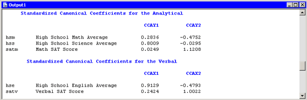
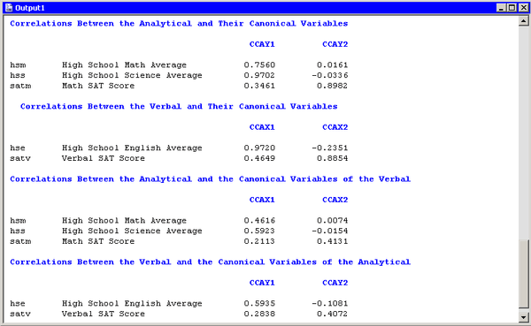
Figure 28.6: Canonical Coefficients

Figure 28.7 displays the table of correlations between the canonical variables and the original variables. These univariate correlations must be interpreted with caution, since they do not indicate how the original variables contribute jointly to the canonical analysis. However, they are often useful in the interpretation of the canonical variables.

The first canonical variable for the analytical group is strongly correlated with hsm and hss, with correlations 0.7560 and 0.9702, respectively. The second canonical variable for the analytical group is strongly correlated with satm, with a correlation of 0.8982.

The first canonical variable for the verbal group is strongly correlated with hse, with a correlation of 0.9720. The second canonical variable for the verbal group is strongly correlated with satv, with a correlation of 0.8854.

Figure 28.7: Correlations between Canonical and Original Variables

In summary, the analytical and verbal variables are moderately correlated with each other, with a canonical correlation of 0.6106. The first canonical variables are close to the linear subspace spanned by the variables that measure a student’s high school grades. The second canonical variables are close to the linear subspace spanned by the SAT variables. (Recall that the span of a set of vectors is the vector space consisting of all linear combinations of the vectors.)