To model Log10_salary as a function of three explanatory variables:
-
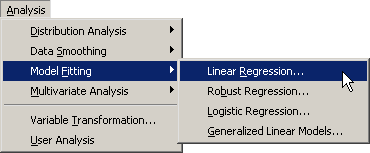
Select → → from the main menu, as shown in Figure 21.5.
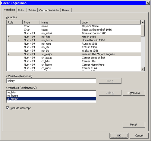
The Linear Regression dialog box appears. (See Figure 21.6.)
-
Scroll to the end of the variable list. Select
Log10_salary, and click . -
Select
no_hits. While holding down the CTRL key, selectno_home, andyr_major. Click . -
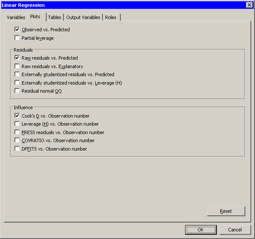
Click the Plots tab.
The Plots tab becomes active, as shown in Figure 21.7. This tab controls which graphs are produced by the analysis.
-
Select .
-
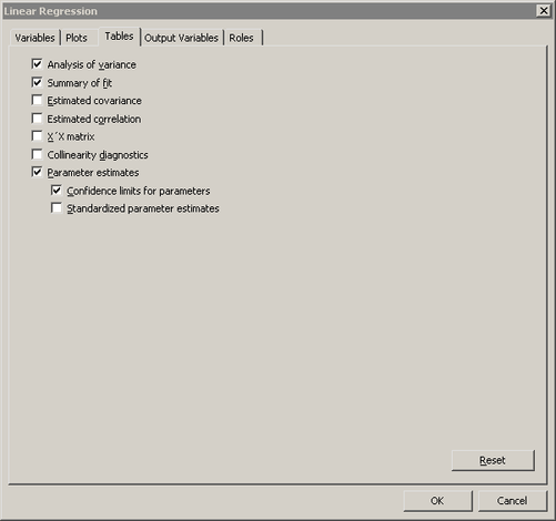
Click the Tables tab.
The Tables tab becomes active, as shown in Figure 21.8.
-
Click .
-
Click .
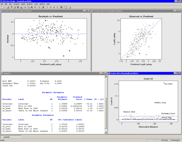
Several plots appear, along with output from the REG procedure. Some plots might be hidden beneath others. Move the windows so that they are arranged as in Figure 21.9.
The Residuals vs. Predicted plot does not show any obvious trends in the residuals, although possibly the residuals are slightly higher for predicted values near the middle of the predicted range. The Observed vs. Predicted plot shows a reasonable fit, with a few exceptions.
In the output window you can see that R square is 0.5646, which means that the model accounts for 56% of the variation in
the data. The no_home term is not significant (![]() ,
, ![]() ) and thus can be removed from the model. This is also seen by noting that the 95% confidence limits for the coefficient of
) and thus can be removed from the model. This is also seen by noting that the 95% confidence limits for the coefficient of
no_home include zero.
The Cook’s ![]() plot shows how deleting any one observation would change the parameter estimates. (Cook’s
plot shows how deleting any one observation would change the parameter estimates. (Cook’s ![]() and other influence statistics are described in the “Influence Diagnostics” section of the documentation for the REG procedure.) A few influential observations have been selected in the plot of Cook’s
and other influence statistics are described in the “Influence Diagnostics” section of the documentation for the REG procedure.) A few influential observations have been selected in the plot of Cook’s
![]() ; these observations are seen highlighted in the other plots. Three players (Steve Sax, Graig Nettles, and Steve Balboni)
with high Cook’s
; these observations are seen highlighted in the other plots. Three players (Steve Sax, Graig Nettles, and Steve Balboni)
with high Cook’s ![]() values also have large negative residuals which indicates that they were paid less than the model predicts.
values also have large negative residuals which indicates that they were paid less than the model predicts.
Two other players (Darryl Strawberry and Pete Rose) are also highlighted. These players are discussed in the next section.