| The PSMOOTH Procedure |
| Statistical Computations |
Methods of Smoothing  -Values
PROC PSMOOTH offers three methods of combining -values over specified sizes of sliding windows. For each value  listed in the BANDWIDTH= option of the PROC PSMOOTH statement, a sliding window of size
  is used; that is, the -values for each set of consecutive markers are considered in turn, for each value . The approach described by Zaykin et al. (2002) is implemented, where the original -value at the center of the sliding window is replaced by a function of the original -value and the -values from the nearest markers on each side to create a new sequence of -values. Note that for markers less than from the beginning or end of the data set (or BY group if any variables are specified in the BY statement), the number of hypotheses tested,
  , is adjusted accordingly. The three methods of combining -values from multiple hypotheses are Simes’ method, Fisher’s method, and the TPM, described in the following three sections. Plotting the new -values versus the original -values reveals the smoothing effect this technique has.
Simes’ Method
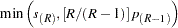
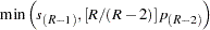
Simes’ method of combining -values (1986) is performed as follows when the SIMES option is specified in the PROC PSMOOTH statement: let  be the original -value at the center of the current sliding window, which contains
  . From these
  -values, the ordered -values,
  are formed. Then the new value for is
  .
.
This method controls the Type I error rate even when hypotheses are positively correlated (Sarkar and Chang 1997), which is expected for nearby markers. Thus if dependencies are suspected among tests that are performed, this method is recommended due to its conservativeness.
Fisher’s Method
When the FISHER option is issued in the PROC PSMOOTH statement, Fisher’s method of combining -values (1932) is applied by replacing the -value at the center of the current sliding window with the -value of the statistic  , where
 |
which has a  distribution under the null hypothesis of all hypotheses being true.
Caution: has a  distribution only under the assumption that the tests performed are mutually independent. When this assumption is violated, the probability of Type I error can exceed the significance level
  .
.
TPM
The TPM is a variation of Fisher’s method that leads to a different alternative hypothesis when  , the value specified in the TAU= option, is less than 1 (Zaykin et al. 2002). With the TPM, rejection of the null hypothesis implies that there is at least one false null hypothesis among those with -values
  . To calculate a combined -value by using the TPM for the -value at the center of the sliding window, , the quantity
  must first be calculated as
 |
Then the formula for the new value for the -value at the center of the sliding window of markers is
 |
When TAU=1 is specified, the TPM and Fisher’s method are equivalent and the previous formula simplifies to
 |
Multiple Testing Adjustments for -Values
While the smoothing methods take into account the -values from neighboring markers, the number of hypothesis tests performed does not change. Therefore, the Bonferroni, false discovery rate (FDR), and Sidak methods are offered by PROC PSMOOTH to adjust the smoothed -values for multiple testing. The number of tests performed,  , is the number of valid observations in the current BY group if any variables are specified in the BY statement, or the number of valid observations in the entire data set if there are no variables specified in the BY statement. Note that these adjustments are not applied to the original column(s) of -values; if you would like to adjust the original -values for multiple testing, you must include a bandwidth of 0 in the BANDWIDTH= option of the PROC PSMOOTH statement along with one of the smoothing methods (SIMES, FISHER, or TPM).
For tests, the -value  results in an adjusted -value of
  according to these methods:
- Bonferroni adjustment:

- Sidak adjustment (Sidak 1967):
- FDR adjustment (Benjamini and Hochberg 1995):


where the -values have been ordered as 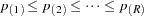 . The Bonferroni and Sidak methods are conservative for controlling the family-wise error rate; however, often in the association mapping of a complex trait, it is desirable to control the FDR instead (Sabatti, Service, and Freimer 2003).
Copyright © 2008 by SAS Institute Inc., Cary, NC, USA. All rights reserved.