The MODEL Procedure
Example 26.21 A Translog Cost Function and Derived Demands
This example shows the use of iterated seemingly unrelated regression (ITSUR) to estimate a system of nonlinear derived demand equations that are based on a translog cost function. Data pertain to the United States textile manufacturing sector (standard industrial classification code 22). The series runs from 1949 to 2001 and contains real quantity indices, price indices, and cost measures for a single aggregate industry output and five aggregate inputs: capital (K), labor (L), energy (E), materials (M), and services (S). The original data and information about other industrial sectors can be obtained from the Multifactor Productivity home page of the Bureau of Labor Statistics at http://www.bls.gov/mfp/.
The demand equations that are derived from the translog cost function are expressed by using a cost share as the endogenous variable. Because these data do not contain explicit information about cost shares, the shares must be formed by taking the ratio of the value of each input and the cost measure. The following statements compute the cost share for each input:
data klems;
set klems;
   array values {5} vk vl ve vm vs;
   array costshares {5} sk sl se sm ss;
   cost = sum(vk,vl,ve,vm,vs);
   do i = 1 to 5;
      costshares{i} = values{i}/cost;
   end;
run;
The following statements produce a time series plot of quantity indices and generate further plots of price indices and cost shares:
   proc sgplot data = klems;
      series x = year y = k / markers markerattrs =(symbol=circle);
      series x = year y = l / markers markerattrs =(symbol=square);
      series x = year y = e / markers markerattrs =(symbol=star);
      series x = year y = m / markers markerattrs =(symbol=diamond);
      series x = year y = s / markers markerattrs =(symbol=hash);
      title 'Factor Quantities';
      yaxis label = 'Quantity';
   run;
Output 26.21.1 shows time series plots of quantity indices, price indices, and cost shares over time, indicating the dynamics of the US textile sector.
Output 26.21.1: Changes in Variables over Time
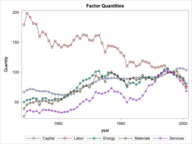
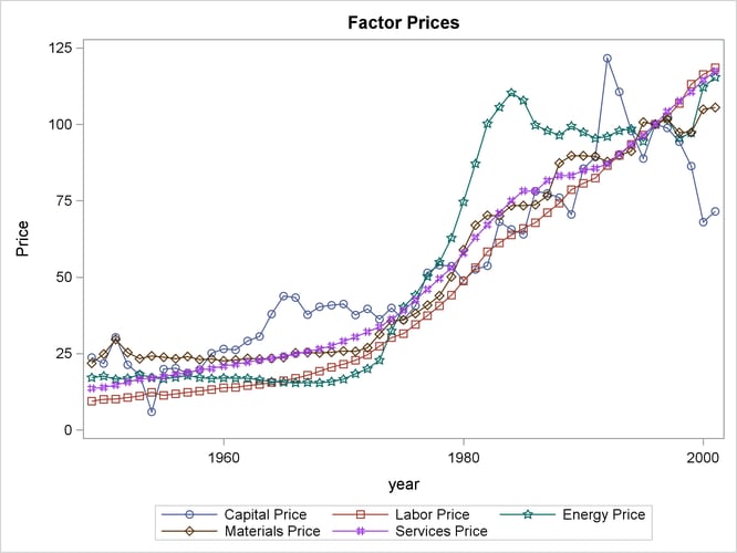
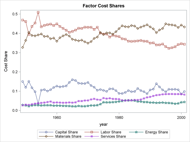
Textile manufacturing was once a significant part of total manufacturing output in the United States. As international trade increased, many textile mills moved overseas, where labor costs are lower than they are in the United States. The first graph in Output 26.21.1 shows that labor use has steadily declined while use of other inputs has grown. Perhaps the textile industry adjusted to foreign competition by increasing use of inputs besides labor. The price of energy increased rapidly in the 1970s, reflecting what has commonly been called the “energy crisis.” As energy prices increased, energy use remained flat or declined. The result of these two movements is a higher cost share for energy in general. As labor use and cost shares declined in the sector, there were nearly coincident increases in the quantity indices and cost shares of capital and purchased services. This relationship suggests that capital and services can substitute for labor in the production of textiles.
Output 26.21.1 does not provide quantifiable measures of the relationship between input use and price or of input substitution. Price elasticities
and substitution elasticities must be calculated from the parameters of the cost function or from factor demands. One benefit
of the translog form is that the system of factor demands produces nearly the same information as the cost function. The only
parameter of the cost function that is not captured by the derived demand system is the intercept term, which is not used
in calculating the desired elasticities. Often, only the system of derived demands is estimated. In this example, the MODEL
procedure is used to fit four derived demand equations. One of the equations (the derived demand equation for services) has
been arbitrarily dropped from estimation; only  of the factor demands are linearly independent because the dependent variables are cost shares, which must sum to one. The
parameters of the dropped derived demand equation can be recovered after estimation through homogeneity and symmetry restrictions.
of the factor demands are linearly independent because the dependent variables are cost shares, which must sum to one. The
parameters of the dropped derived demand equation can be recovered after estimation through homogeneity and symmetry restrictions.
The following statements estimate the system of derived demand equations without imposing any restrictions. Likelihood ratio tests are performed to determine whether homogeneity and symmetry restrictions hold both singularly and jointly.
   proc model data = klems;
      parameters a_k gkk gkl gke gkm gks gky
                 a_l glk gll gle glm gls gly
                     a_e gek gel gee gem ges gey
                     a_m gmk gml gme gmm gms gmy;
      endogenous sk sl se sm;
      exogenous pk pl pe pm ps y;

      /*System of Derived Demand Equations*/
      sk = a_k + gkk*log(pk) + gkl*log(pl) + gke*log(pe) + gkm*log(pm) + gks*log(ps)
               + gky*log(y);
      sl = a_l + glk*log(pk) + gll*log(pl) + gle*log(pe) + glm*log(pm) + gls*log(ps)
               + gly*log(y);
      se = a_e + gek*log(pk) + gel*log(pl) + gee*log(pe) + gem*log(pm) + ges*log(ps)
               + gey*log(y);
      sm = a_m + gmk*log(pk) + gml*log(pl) + gme*log(pe) + gmm*log(pm) + gms*log(ps)
               + gmy*log(y);

      fit sk sl se sm / itsur;

      test "Homogeneity"
         gkk+gkl+gke+gkm+gks=0,
         glk+gll+gle+glm+gls=0,
         gek+gel+gee+gem+ges=0,
         gmk+gml+gme+gmm+gms=0, / lr;

      test "Symmetry"
         gkl=glk,
         gke=gek,
         gkm=gmk,
         glm=gml,
         gle=gel,
         gem=gme, / lr;

      test "Joint Homogeneity and Symmetry"
         gkk+gkl+gke+gkm+gks=0,
         glk+gll+gle+glm+gls=0,
         gek+gel+gee+gem+ges=0,
         gmk+gml+gme+gmm+gms=0,
         gkl=glk,
         gke=gek,
         gkm=gmk,
         glm=gml,
         gle=gel,
         gem=gme, / lr;
   run;
The summary of residual errors provides fit statistics for each of the estimated demand equations and is shown in Output 26.21.2. In this case, the model fits the data well based on R-squared values.
Output 26.21.2: Residual Summary
| Nonlinear ITSUR Summary of Residual Errors | ||||||||
|---|---|---|---|---|---|---|---|---|
| Equation | DF Model | DF Error | SSE | MSE | Root MSE | R-Square | Adj R-Sq | Label |
| sk | 7 | 46 | 0.00118 | 0.000026 | 0.00506 | 0.9519 | 0.9457 | Capital Share |
| sl | 7 | 46 | 0.00449 | 0.000098 | 0.00988 | 0.9565 | 0.9508 | Labor Share |
| se | 7 | 46 | 0.000079 | 1.724E-6 | 0.00131 | 0.9847 | 0.9827 | Energy Share |
| sm | 7 | 46 | 0.00436 | 0.000095 | 0.00973 | 0.9146 | 0.9035 | Materials Share |
Because the form of the elasticities is somewhat complicated, it can be difficult to interpret the values and signs of parameter estimates. It is far easier to compute the elasticities directly. The test results in Output 26.21.3 indicate that both symmetry and homogeneity are rejected. A common practice is to assume that such restrictions hold and to impose them in estimation.
Output 26.21.3: Tests of Symmetry and Homogeneity
| Test Results | ||||
|---|---|---|---|---|
| Test | Type | Statistic | Pr > ChiSq | Label |
| Homogeneity | L.R. | 114.22 | <.0001 | gkk+gkl+gke+gkm+gks=0, glk+gll+gle+glm+gls=0, gek+gel+gee+gem+ges=0, gmk+gml+gme+gmm+gms=0 |
| Symmetry | L.R. | 109.72 | <.0001 | gkl=glk, gke=gek, gkm=gmk, glm=gml, gle=gel, gem=gme |
| Joint Homogeneity and Symmetry | L.R. | 240.80 | <.0001 | gkk+gkl+gke+gkm+gks=0, glk+gll+gle+glm+gls=0, gek+gel+gee+gem+ges=0, gmk+gml+gme+gmm+gms=0, gkl=glk, gke=gek, gkm=gmk, glm=gml, gle=gel, gem=gme |
The following code imposes both symmetry and homogeneity restrictions on the underlying model:
   proc model data = klems;
       parameters a_k gkk gkl gke gkm gks gky
                  a_l glk gll gle glm gls gly
                  a_e gek gel gee gem ges gey
                  a_m gmk gml gme gmm gms gmy;
       endogenous sk sl se sm;
       exogenous pk pl pe pm ps y;
       restrict /*Homogeneity Restrictions*/
                gks+gkk+gkl+gke+gkm=0,
                gls+gkl+gll+gle+glm=0,
                ges+gke+gle+gee+gem=0,
                gms+gkm+glm+gem+gmm=0,
                /*Symmetry Restrictions*/
                gkl=glk, gke=gek, gkm=gmk, gle=gel, glm=gml, gem=gme;

       /*System of Derived Demand Equations*/
       sk = a_k + gkk*log(pk) + gkl*log(pl) + gke*log(pe) + gkm*log(pm) + gks*log(ps)
                + gky*log(y);
       sl = a_l + glk*log(pk) + gll*log(pl) + gle*log(pe) + glm*log(pm) + gls*log(ps)
                + gly*log(y);
       se = a_e + gek*log(pk) + gel*log(pl) + gee*log(pe) + gem*log(pm) + ges*log(ps)
                + gey*log(y);
       sm = a_m + gmk*log(pk) + gml*log(pl) + gme*log(pe) + gmm*log(pm) + gms*log(ps)
                + gmy*log(y);

       fit sk sl se sm / itsur chow = (24) outest=est;

       test "Constant Returns to Scale"
          gky=0,
          gly=0,
          gey=0,
          gmy=0, / lr;
   run;
The symmetry restriction shrinks the number of parameters of the model considerably. This shrinkage is particularly useful when the time series is not long and degrees of freedom need to be conserved. Output 26.21.4 shows the parameter estimates of the MODEL procedure.
Output 26.21.4: Restricted Model
| Nonlinear ITSUR Parameter Estimates | |||||
|---|---|---|---|---|---|
| Parameter | Estimate | Approx Std Err | t Value | Approx Pr > |t| |
Label |
| a_k | 0.109996 | 0.0219 | 5.02 | <.0001 | SK Intercept |
| gkk | 0.062014 | 0.00357 | 17.38 | <.0001 | SK K Price |
| gkl | -0.01898 | 0.00725 | -2.62 | 0.0118 | SK L Price |
| gke | -0.00179 | 0.000836 | -2.15 | 0.0369 | SK E Price |
| gkm | -0.03872 | 0.00610 | -6.35 | <.0001 | SK M Price |
| gks | -0.00252 | 0.00342 | -0.74 | 0.4648 | SK S Price |
| gky | -0.00104 | 0.00496 | -0.21 | 0.8354 | SK Output |
| a_l | 0.865473 | 0.0903 | 9.58 | <.0001 | SL Intercept |
| glk | -0.01898 | 0.00725 | -2.62 | 0.0118 | SL K Price |
| gll | -0.00999 | 0.0360 | -0.28 | 0.7826 | SL L Price |
| gle | -0.00106 | 0.00420 | -0.25 | 0.8013 | SL E Price |
| glm | -0.06766 | 0.0248 | -2.73 | 0.0087 | SL M Price |
| gls | 0.097692 | 0.0214 | 4.57 | <.0001 | SL S Price |
| gly | -0.11488 | 0.0200 | -5.74 | <.0001 | SL Output |
| a_e | 0.012747 | 0.00984 | 1.30 | 0.2013 | SE Intercept |
| gek | -0.00179 | 0.000836 | -2.15 | 0.0370 | SE K Price |
| gel | -0.00106 | 0.00420 | -0.25 | 0.8013 | SE L Price |
| gee | 0.029876 | 0.00112 | 26.76 | <.0001 | SE E Price |
| gem | -0.01954 | 0.00275 | -7.12 | <.0001 | SE M Price |
| ges | -0.00748 | 0.00325 | -2.30 | 0.0257 | SE S Price |
| gey | 0.005808 | 0.00217 | 2.68 | 0.0101 | SE Output |
| a_m | -0.08173 | 0.0701 | -1.17 | 0.2492 | SM Intercept |
| gmk | -0.03872 | 0.00610 | -6.35 | <.0001 | SM K Price |
| gml | -0.06766 | 0.0248 | -2.73 | 0.0087 | SM L Price |
| gme | -0.01954 | 0.00275 | -7.12 | <.0001 | SM E Price |
| gmm | 0.146849 | 0.0222 | 6.62 | <.0001 | SM M Price |
| gms | -0.02092 | 0.0103 | -2.03 | 0.0477 | SM S Price |
| gmy | 0.113729 | 0.0157 | 7.27 | <.0001 | SM Output |
| Restrict0 | -563.453 | 242.8 | -2.32 | 0.0187 | gks+gkk+gkl+gke+gkm=0 |
| Restrict1 | 82.23307 | 193.0 | 0.43 | 0.6747 | gls+gkl+gll+gle+glm=0 |
| Restrict2 | 321.7446 | 689.2 | 0.47 | 0.6455 | ges+gke+gle+gee+gem=0 |
| Restrict3 | -279.71 | 211.0 | -1.33 | 0.1879 | gms+gkm+glm+gem+gmm=0 |
| Restrict4 | -261.228 | 196.3 | -1.33 | 0.1860 | gkl=glk |
| Restrict5 | -1041.84 | 755.0 | -1.38 | 0.1700 | gke=gek |
| Restrict6 | -27.855 | 219.3 | -0.13 | 0.9005 | gkm=gmk |
| Restrict7 | -880.821 | 742.7 | -1.19 | 0.2396 | gle=gel |
| Restrict8 | 259.513 | 215.6 | 1.20 | 0.2326 | glm=gml |
| Restrict9 | 1103.343 | 320.8 | 3.44 | 0.0003 | gem=gme |
The majority of the parameter estimates are significant, and insignificant parameters are statistically equivalent to 0. When
the  are all 0, the translog cost function reduces to the Cobb-Douglas cost function. Statistically insignificant parameter estimates
imply that corresponding elasticities of substitution are equal to the Cobb-Douglas value of 1.
are all 0, the translog cost function reduces to the Cobb-Douglas cost function. Statistically insignificant parameter estimates
imply that corresponding elasticities of substitution are equal to the Cobb-Douglas value of 1.
A TEST statement is used to determine whether this industry exhibits constant returns to scale in the range of the sample. The CHOW option in the FIT statement performs a Chow test for a structural break at the 24th year of the sample (1973). In October of that year the Organization of Petroleum Exporting Countries (OPEC) declared an oil embargo. Markets were affected by significant shocks to oil prices, and gasoline in the United States was rationed. Output 26.21.5 shows the results of the two tests.
Output 26.21.5: CRS and Chow Test Results
The null hypothesis of constant returns to scale is rejected. The null hypothesis of the Chow test cannot be rejected. Even with the turmoil of the oil embargo, there is no evidence of a structural break in 1973.
Derivations of the Hicks-Allen elasticity of substitution, the Morishima elasticity of substitution, and the price elasticity of demand for the translog cost function can be found in Chambers (1988). The elasticities are evaluated at the sample mean, so the MEANS procedure is used in the following statements to produce data that contain the sample means of the cost shares:
proc means data = klems noprint mean;
   variables sk sl se sm ss;
   output out = meanshares mean = sk sl se sm ss;
run;
Because some of the parameters are not estimated, their values must be backed out through application of homogeneity and symmetry restrictions. The IML procedure is used in the following statements to read in parameter estimates and then calculate elasticities:
   proc iml;
      /*Read in parameter estimates*/
      use est;
      read all var {gkk gkl gke gkm gks};
      read all var {gll gle glm gls};
      read all var {gee gem ges};
      read all var {gmm gms};
      close est;

      /*Calculate S parameter based on homogeneity constraint*/
      gss=0-gks-gls-ges-gms;

      /*Read in mean cost shares and construct vector*/
      use meanshares;
      read all var {sk sl se sm ss};
      close meanshares;

      w = sk//sl//se//sm//ss;

     print w;

     /*Construct matrix of parameter estimates*/
     gij = (gkk||gkl||gke||gkm||gks)//
           (gkl||gll||gle||glm||gls)//
           (gke||gle||gee||gem||ges)//
           (gkm||glm||gem||gmm||gms)//
           (gks||gls||ges||gms||gss);

      print gij;

      nk=ncol(gij);
      mi = -1#I(nk);    /*Initialize negative identity matrix*/
      eos = j(nk,nk,0); /*Initialize Marshallian EOS Matrix*/
      mos = j(nk,nk,0); /*Initialize Morishima EOS Matrix*/
      ep  = j(nk,nk,0); /*Initialize Price EOD Matrix*/

      /*Calculate Marshallian EOS and Price EOD Matrices*/
      i=1;
      do i=1 to nk;
      j=1;
      do j=1 to nk;
          eos[i,j] = (gij[i,j]+w[i]#w[j]+mi[i,j]#w[i])/(w[i]#w[j]);
          ep[i,j] = w[j]#eos[i,j];
      end;
      end;

      /*Calculate Morishima EOS Matrix*/
      i=1;
      do i=1 to nk;
      j=1;
      do j=1 to nk;
         mos[i,j] = ep[i,j]-ep[j,j];
      end;
      end;

   run;
Output 26.21.6 shows the elasticity matrices that are generated by the IML procedure.
Output 26.21.6: Elasticity Matrices
Own price elasticities are all negative as expected. Based on the price elasticity of demand, all pairs of inputs are substitutes except energy and services and energy and materials. The matrix of Hicks-Allen elasticities is symmetric by design. In general, most of the elasticities are less than 1 in absolute value and the degree of substitution is low. However, the elasticity between labor and services is high, indicating that the textile industry might have responded to increased competition from foreign firms that have low labor cost by shifting away from labor to greater use of services. The Morishima elasticities support this interpretation, but there are subtle differences between the two measures. The relationship between capital and services is more elastic when the Morishima elasticity is used. The estimation of elasticities thoroughly describes production in this industry and produces quantifiable measures of the relationships between inputs.