The MODEL Procedure
Solution Mode Output
The following SAS statements dynamically forecast the solution to a nonlinear equation:
proc model data=sashelp.citimon;
   parameters a 0.010708  b  -0.478849 c 0.929304;
   lhur = 1/(a * ip) + b + c * lag(lhur);
   solve lhur / out=sim forecast dynamic;
run;
The first page of output produced by the SOLVE step is shown in Figure 26.77. This is the summary description of the model. The error message states that the simulation was aborted at observation 144 because of missing input values.
Figure 26.77: Solve Step Summary Output
The second page of output, shown in Figure 26.78, gives more information on the failed observation.
Figure 26.78: Solve Step Error Message
| Solution values are missing because of missing input values for observation 144 at NEWTON iteration 0. |
| Note: | Additional information on the values of the variables at this observation, which may be helpful in determining the cause of the failure of the solution process, is printed below. |
| Observation | 144 | Iteration | 0 | CC | -1.000000 |
|---|---|---|---|---|---|
| Missing | 1 |
From the program data vector, you can see the variable IP is missing for observation 144. LHUR could not be computed, so the simulation aborted.
The solution summary table is shown in Figure 26.79.
Figure 26.79: Solution Summary Report
This solution summary table includes the names of the input data set and the output data set followed by a description of the model. The table also indicates that the solution method defaulted to Newton’s method. The remaining output is defined as follows.
|
Maximum CC |
is the maximum convergence value accepted by the Newton |
|
procedure. This number is always less than the value |
|
|
for the CONVERGE= option. |
|
|
Maximum Iterations |
is the maximum number of Newton iterations performed |
|
at each observation and each replication of Monte |
|
|
Carlo simulations. |
|
|
Total Iterations |
is the sum of the number of iterations required for each |
|
observation and each Monte Carlo simulation. |
|
|
Average Iterations |
is the average number of Newton iterations required to |
|
solve the system at each step. |
|
|
Solved |
is the number of observations used times the number of |
|
random replications selected plus one, for Monte Carlo |
|
|
simulations. The one additional simulation is the original |
|
|
unperturbed solution. For simulations that do not involve Monte |
|
|
Carlo, this number is the number of observations used. |
Summary Statistics
The STATS and THEIL options are used to select goodness-of-fit statistics. Actual values must be provided in the input data set for these statistics to be printed. When the RANDOM= option is specified, the statistics do not include the unperturbed (_REP_=0) solution.
STATS Option Output
The following statements show the addition of the STATS and THEIL options to the model in the previous section:
proc model data=sashelp.citimon;
   parameters a 0.010708  b  -0.478849 c 0.929304;
   lhur= 1/(a * ip) + b + c * lag(lhur) ;
   solve lhur / out=sim dynamic stats theil;
   range date to '01nov91'd;
run;
The STATS output in Figure 26.80 and the THEIL output in Figure 26.81 are generated.
Figure 26.80: STATS Output
The number of observations (Nobs), the number of observations with both predicted and actual values nonmissing (N), and the mean and standard deviation of the actual and predicted values of the determined variables are printed first. The next set of columns in the output are defined as follows:
|
Mean Error |
|
|
Mean % Error |
|
|
Mean Abs Error |
|
|
Mean Abs % Error |
|
|
RMS Error |
|
|
RMS % Error |
|
|
R-square |
|
|
SSE |
|
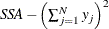
|
SSA |
|
|
CSSA |
|
|
|
predicted value |
|
y |
actual value |

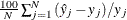

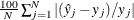
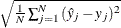
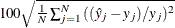


When the RANDOM= option is specified, the statistics do not include the unperturbed (_REP_=0) solution.
THEIL Option Output
The THEIL option specifies that Theil forecast error statistics be computed for the actual and predicted values and for the relative changes from lagged values. Mathematically, the quantities are
![\[ \hat{yc} = (\hat{y} - lag(y)) / lag(y) \]](images/etsug_model0576.png)
![\[ yc = (y - lag(y)) / lag(y) \]](images/etsug_model0577.png)
where  is the relative change for the predicted value and
  is the relative change for the actual value.
Figure 26.81: THEIL Output
The columns have the following meaning:
- Corr (R)
-
is the correlation coefficient,
 , between the actual and predicted values.
![\[ {\rho } = \frac{\mr{cov}( y, \hat{y})}{ {\sigma }_{a} {\sigma }_{p}} \]](images/etsug_model0581.png)
where
 and
and  are the standard deviations of the predicted and actual values.
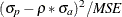
- Bias (UM)
-
is an indication of systematic error and measures the extent to which the average values of the actual and predicted deviate from each other.
![\[ \frac{(\mr{E}(y)- \mr{E}(\hat{y}))^{2}}{ \frac{1}{N} \sum _{t=1}^{N}{(y_{t} - \hat{y}_{t})^{2}}} \]](images/etsug_model0584.png)
- Reg (UR)
-
is defined as
 . Consider the regression
![\[ y = {\alpha }+ {\beta }\hat{y} \]](images/etsug_model0586.png)
If
 , UR will equal zero.
- Dist (UD)
-
is defined as
 and represents the variance of the residuals obtained by regressing on .
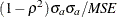
- Var (US)
-
is the variance proportion. US indicates the ability of the model to replicate the degree of variability in the endogenous variable.
![\[ \mi{US} = \frac{({\sigma }_{p}-{\sigma }_{a})^{2}}{\mi{MSE}} \]](images/etsug_model0589.png)
- Covar (UC)
-
represents the remaining error after deviations from average values and average variabilities have been accounted for.
![\[ \mi{UC} = \frac{2(1 - {\rho }) {\sigma }_{p}{\sigma }_{a}}{\mi{MSE}} \]](images/etsug_model0590.png)
- U1
-
is a statistic that measures the accuracy of a forecast defined as follows:
![\[ \mi{U1} =\frac{\sqrt {\mi{MSE}}}{\sqrt {\frac{1}{N}\sum _{t=1}^{N}{(y_{t})^{2}}}} \]](images/etsug_model0591.png)
- U
-
is the Theil’s inequality coefficient defined as follows:
![\[ \mi{U} = \frac{\sqrt {\mi{MSE}}}{\sqrt {\frac{1}{N}\sum _{t=1}^{N}{(y_{t})^{2}}} + \sqrt {\frac{1}{N}\sum _{t=1}^{N}{( \hat{y}_{t})^{2}}}} \]](images/etsug_model0592.png)
- MSE
-
is the mean square error. In the case of the relative change Theil statistics, the MSE is computed as follows:
![\[ \mi{MSE} = \frac{1}{N} \sum _{t=1}^{N}{(\hat{yc}_ t - yc_ t)^{2}} \]](images/etsug_model0593.png)
More information about these statistics can be found in the references Maddala (1977, pp. 344–347) and Pindyck and Rubinfeld (1981, pp. 364–365).